
Apparently, CloudLinux recently accidentally released a non-GPLed driver that still used GPL-only kernel symbols, and that claimed to the kernel to be GPLed code. Matthew Garrett noticed this first, and submitted a patch to cause the kernel to treat the module as non-GPL automatically and deny it access to the GPL-only symbols. Because the violation was so blatant, a number of kernel developers seemed to favor potentially taking legal action against CloudLinux. Greg Kroah-Hartman was particularly dismayed, since the driver in question used kernel symbols he himself had created for GPL use only.
At one point the CEO of CloudLinux, Igor Seletskiy, explained that this just had been an engineering mistake. They had decided to release their GPLed driver under a proprietary license, which as the copyright holders they were allowed to do, but they mistakenly had failed to update the code to stop using GPL-only symbols. He promised to fix the problem within the next few weeks and to provide source code to the binary driver that had caused the fuss.
Chris Jones recently asked what the etiquette was for giving his own personal version numbers to his own customized kernels. Greg Kroah-Hartman replied that he was free to do whatever he wanted in that arena without offending anyone. But, Greg suggested that in order for Chris' users to be able to understand the features and capabilities of the particular customized kernels, Chris probably would be served best by relying on the official version numbers and just appending his own afterward—for example, Linux version 3.4-cj2.
Apparently, the number of patch submissions coming into the Linux kernel is in the process of exploding at the speed of light, like a new Big Bang. Thomas Gleixner remarked on this trend and suggested that the kernel development process might have to be modified to be able to handle such an E=mc2-esque situation. Greg Kroah-Hartman even said he thought the increase in patch submissions might be an intentional denial-of-service attack, designed to interfere with the ability of the kernel developers to keep developing. Thomas didn't think this was likely, but he did point out that a number of companies assessed the performance of their kernel-hacking employees by the number of patches accepted into the kernel, or the total number of lines of code going into the tree. He speculated that this type of performance evaluation, implemented by companies around the world, might account for the DoS-seeming nature of the situation.
Thomas Gleixner pointed out that there was a problem with kernel code maintainers who pushed their own agendas too aggressively and ignored their critics just because they could get away with it. Greg Kroah-Hartman agreed that this was a tough problem to solve, but he added that in the past, problem maintainers seemed to go away on their own after a while. Alan Cox said that in his opinion, maintainers who seemed to be pushing their own agendas were really just doing development the way they thought it should be done, which was what a maintainer should be doing.
But, Alan did agree that maintainers sometimes were lax on the job, because of having children or illnesses or paid employment in other fields. He suggested that having co-maintainers for any given area of code might be a good way to take up some of the slack.
Another idea, from Trond Myklebust, was to encourage maintainers to insist on having at least one “Reviewed-By” tag on each patch submission coming in, so that anyone sending in a patch would be sure to run it by at least one other person first. That, he said, could have the effect of reducing the number of bad patches coming in and easing the load on some of the maintainers.
High-energy physics experiments tend to generate huge amounts of data. While this data is passed through analysis software, very often the first thing you may want to do is to graph it and see what it actually looks like. To this end, a powerful graphing and plotting program is an absolute must. One available package is called Extrema (exsitewebware.com/extrema/index.html). Extrema evolved from an earlier software package named Physica. Physica was developed at the TRIUMF high-energy centre in British Columbia, Canada. It has both a complete graphical interface for interactive use in data analysis and a command language that allows you to process larger data sets or repetitive tasks in a batch fashion.
Installing Extrema typically is simply a matter of using your distribution's package manager. If you want the source, it is available at the SourceForge site (sourceforge.net/projects/extrema). At SourceForge, there also is a Windows version, in case you are stuck using such an operating system.
Once it is installed on your Linux box, launching it is as simple as typing in extrema and pressing Enter. At start up, you should see two windows: a visualization window and an analysis window (Figure 1). One of the most important buttons is the help button. In the analysis window, you can bring it up by clicking on the question mark (Figure 2). In the help window, you can get more detailed information on all the functions and operators available in Extrema.
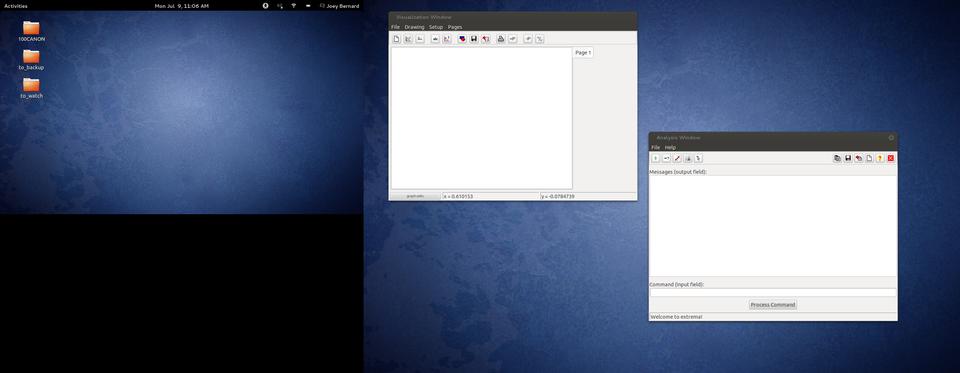
Figure 1. On startup, you are presented with a blank visualization window and an analysis window.
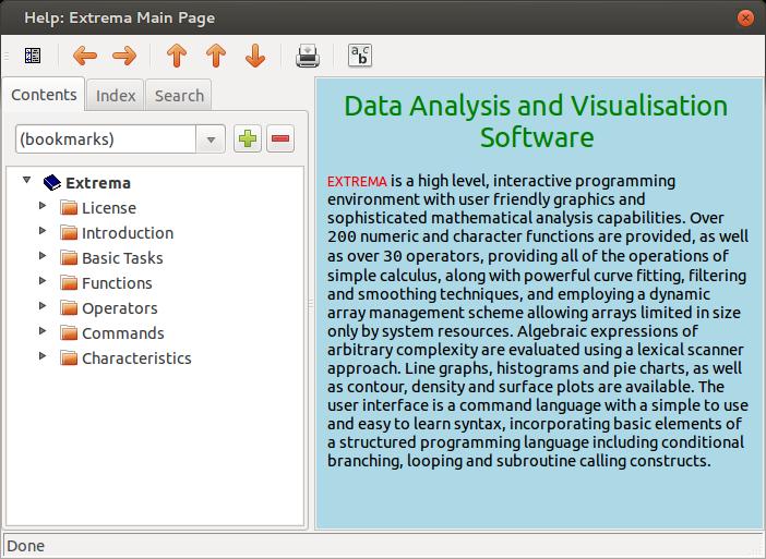
Figure 2. The help window gives you information on all of the available functions, operators and commands.
Extrema provides 3-D contour and density plots. For 2-D graphing, you can control almost all the features, like axes, plot points, colors, fonts and legends. You also can do some data analysis from within Extrema. You can do various types of interpolation, such as linear, Lagrange or Fritsch-Carlson. You can fit an equation to your data with up to 25 parameters. Extrema contains a full scripting language that includes nested loops, branches and conditional statements. You either can write out scripts in a text editor or use the automatic script-writing mode that translates your point-and-click actions to the equivalent script commands.
The first thing you will need to do is get your data into Extrema. Data is stored in variables and is referenced by the variable's name. The first character of a variable name must be alphabetic and cannot be any longer than 32 characters. Other than these restrictions, variable names can contain any alphabetic or numeric characters, underscores or dollar signs. Unlike most things in Linux, variable names are case-insensitive. And remember, function names are reserved, so you can't use them as variable names.
String variables can contain either a single string of text or an array of text strings. Numeric variables can contain a single number, a vector (1-D array), a matrix (2-D array) or a tensor (3-D array). All numbers are stored as double-precision real values. Unlike most other programming languages, these arrays are indexed starting at 1, rather than 0. There are no limits to the size of these arrays, other than the amount of memory available on your machine. Indexing arrays in Extrema can be interesting. If you want the eighth element of array x, you simply can reference it with x[8]. You can grab elements 8, 9 and 10 with x[8:10]. These indices can be replaced with expressions, so you could get the eighth element with x[2^3].
There also are special characters that you can use in indexing arrays. The statement x[*] refers to all the values in the vector. If you want the last element, you can use x[#]. The second-to-last element can be referenced with x[#-1].
You likely have all of your data stored in files. The simplest file format is a comma-separated list of values. Extrema can read in these types of files and store the data directly into a set of variables. If you have a file with two columns of data, you can load them into two variables with the statement:
READ file1.dat x y
You also can read in all of the data and store it into a single matrix with:
READ\matrix file1.dat m nrows
In order to do this, you need to provide the number of rows that are being read in. You also can generate data to be used in your analysis. If you simply need a series of numbers, you can use:
x = [startval:stopval:stepsize]
This will give you an array of numbers starting at startval, incrementing by stepsize until you reach stopval. You can use the GENERATE command to do this as well. The GENERATE command also will generate an array of random numbers with:
GENERATE\RANDOM x min max num_points
Extrema has all of the standard functions available, like the various types of trigonometric functions. The standard arithmetic operators are:
+ — addition
- — subtraction
* — multiplication
/ — division
^ — exponentiation
() — grouping of terms
There also are special operators for matrix and vector operations:
>< — outer product
<> — inner product
<- — matrix transpose
>- — matrix reflect
/| — vector union
/& — vector intersection
There also is a full complement of logical Boolean operators that give true (1) or false (0) results.
Now that you have your data and have seen some of the basic functions and operators available, let's take a look at graphing this data and doing some analysis on it. The most basic type of graph is plotting a one-dimensional array. When you do this, Extrema treats the data as the y value and the array index as the x value. To see this in action, you can use:
x = [1:10:1]
GRAPH x
This plots a fairly uninteresting straight line (Figure 3).
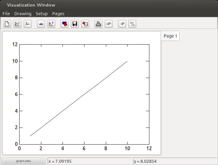
Figure 3. Plotting a Vector of Values
To plot two-dimensional data, you can use:
GRAPH x y
where x and y are two vectors of equal length. The default is to draw the data joined by a solid line. If you want your data as a series of disconnected points, you can set the point type to a negative number, for example:
SET PLOTSYMBOL -1
Then you can go ahead and graph your data.
Parametric plots also are possible. Let's say you have an independent variable called t that runs from 0 to 2*Pi. You then can plot t*sin(t) and t*cos(t) with:
t = [0:2*pi:0.1]
x = t * sin(t)
y = t * cos(t)
graph x y
This will give you the plot shown in Figure 4.
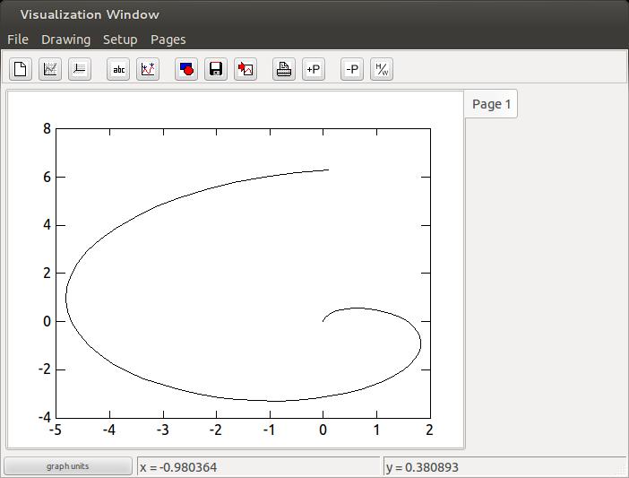
Figure 4. Graphing a Parametric Plot
In scientific experiments, you usually have some value for error in your measurements. You can include this in your graphs as an extra parameter to the graph command, assuming these error values are stored in an extra variable. So, you could use:
graph x y yerr
to get a nice plot. Many options are available for the graph command (Figure 5).
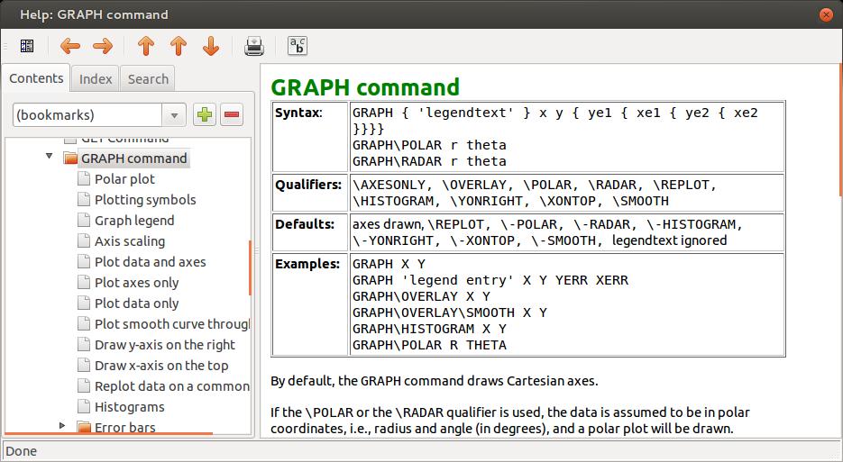
Figure 5. The graph command has many available options.
More complicated data can be graphed in three dimensions. There are several types of 3-D graphs, including contour plots and surface plots. The simplest data structure would be a matrix, where the indices represent the x and y values, and the actual numbers in the matrix are the z values. If this doesn't work, you can represent the separate x, y and z values with three different vectors, all of the same length. The most basic contour graph can be made with the command:
CONTOUR m
where m is the matrix of values to be graphed. In this case, Extrema will make a selection of “nice” contour lines that create a reasonable graph.
You can draw a density plot of the same data with the density command, where the values in your matrix are assigned a color from a color map, and that is what gets graphed. Unless you say differently, Extrema will try to select a color map that fits your data the best. A surface plot tries to draw a surface in the proper perspective to show what surface is defined by the z values in your data.
Let's finish by looking at one of the more important analysis steps, fitting an equation to your data. The point of much of science is to develop equations that describe the data being observed, in the hope that you then will be able to predict what you would see under different conditions. Also, you may learn some important underlying physics by looking at the structure of the equation that fits your data. Let's look at a simple fitting of a straight line. Let's assume that the data is stored in two vectors called x and y. You'll also need two other variables to store the slope and intercept. Let's call them b and a. Then you can fit your data with the command:
SCALAR\FIT a b
FIT y=a+b*x
Then, if you want to graph your straight line fit and your data, you can do something like:
SET PLOTSYMBOL -1
SET PLOTSYMBOLCOLOR RED
GRAPH x y
SET PLOTSYMBOL 0
SET CURVECOLOR BLUE
GRAPH x a+b*x
Now that you have seen the basics of what Extrema can do, hopefully you will be inspired to explore it further. It should be able to meet most of your data-analysis needs, and you can have fun using the same tool that is being used by leading particle physicists.
The concept of standalone Web apps isn't new. Anyone using Prism with Firefox or Fluid with OS X understands the concept: a browser that goes to a single Web site and acts like a standalone application—sorta.

With Fogger, however, Web applications take on a whole new meaning. Using a variety of desktop APIs and user scripts, applications created with the Fogger framework integrate into the Linux desktop very much like a traditional application. If you've ever found Web apps to be lacking, take a look at Fogger; it makes the Web a little easier to see: https://launchpad.net/fogger.
As a LibreOffice user, and an OpenOffice.org user before that, the idea of printing to a PDF is nothing new. If you're stuck on a Windows machine, however, it's not always easy to “be green” by printing to a digital file. Thankfully, there's the trusty PDFCreator package. PDFCreator installs like any other program in Windows and then creates a virtual printer that any program can use to generate PDF files.
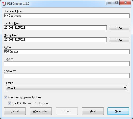
(Image from www.pdfforge.org)
As it has matured, PDFCreator has gained a bunch of neat features. Whether you want to e-mail your PDF files directly, sign them digitally or even encrypt them, PDFCreator is a great tool. Check it out at www.pdfforge.org.
I often discuss the Linux port of Scrivener with my writer friend Ken McConnell. We both like Scrivener's interface, and we both prefer to use Linux as our writing platform. Unfortunately, the Linux port of Scrivener just doesn't compare to the OS X version. The other day, Ken told me about Plume Creator.
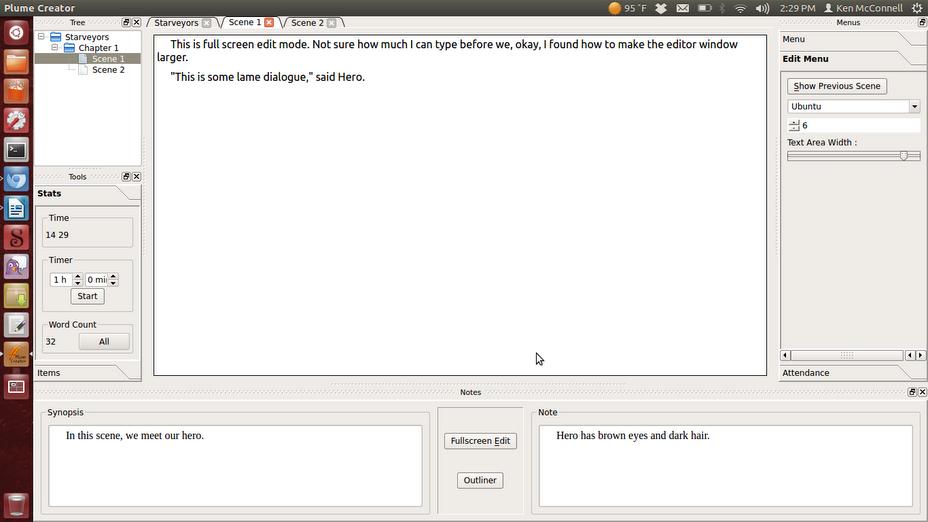
(Image Courtesy of www.ken-mcconnell.com)
With a very similar interface, Plume Creator will feel quite familiar to any Scrivener user. It's very early in development, but it already behaves much nicer than the Linux port of Scrivener. If you've ever wanted to write a novel, or even considered giving NaNoWriMo (www.nanowrimo.org) a try, Plume Creator is worth a look. Get it today at plume-creator.sf.net.
If you've ever run Valve Software's Steam client on your Linux box using Wine, you know that even if you pretend it works well, it really doesn't. Wouldn't it be great if Valve finally would release a native client for Linux? Thankfully, Valve agrees! On a recent blog post (blogs.valvesoftware.com/linux/steamd-penguins) the Valve folks verify that they're creating a native Ubuntu 12.04 Steam client. It's bad news for zombies, however, because the first game they're porting to the penguin platform is Left For Dead 2.

Granted, the Steam client alone doesn't mean the Linux game library will explode overnight, but it does mean game developers will have one more reason to take Linux users seriously. There have been rumors of Steam for Linux for years, but this time, it looks like it really will happen! Stay tuned to the Valve blog for more details.
I don't believe in e-mail. I rarely use a cell phone and I don't have a fax.
—Seth Green
I was just in the middle of singing a song about how broke we were and now my cell phone rings.
—Joel Madden
To be happy in this world, first you need a cell phone and then you need an airplane. Then you're truly wireless.
—Ted Turner
You have to take into account it was the cell phone that became what the modern-day concept of a phone call is, and this is a device that's attached to your hip 24/7. Before that there was “leave a message” and before that there was “hopefully you're home”.
—Giovanni Ribisi
You want to see an angry person? Let me hear a cell phone go off.
—Jim Lehrer