
David Herrmann wanted to disable the virtual terminal subsystem in order to save space on a kernel that didn't need a VT. But, he still wanted to see kernel oops output for debugging purposes. The problem was that only the VT subsystem would display oops output—and he'd just disabled it.
No problem. David posted a patch to implement DRM-log, a separate console device that used the direct rendering manager and that could receive kernel oops output.
Over the course of a discussion about the patch, Alan Cox mentioned that there didn't seem to be anything particularly DRM-specific in David's code. It easily could exist at a yet more generic layer of the kernel. And although David agreed with this, he said the DRM folks were more amenable to taking his patch and that “I've spent enough time trying to get the attention of core maintainers for simple fixes, I really don't want to waste my time pinging on feature-patches every 5 days to get any attention. If someone outside of DRM wants to use it, I'd be happy to discuss any code-sharing. Until then, I'd like to keep it here as people are willing to take it through their tree.”
That's a fairly surprising statement—a bit of an indictment of existing kernel patch submission processes. There was no further discussion on that particular point, but I would imagine it got some folks thinking.
The rest of the current thread focused on some technical details about oops output, especially font size. David's code displayed oops output pixel by pixel, essentially defining its own font. But for extremely high-resolution monitors, such as Apple's Retina display, as Bruno Prémont pointed out, this could result in the oops output being too small for the user to see.
David's answer to this was to implement integer scaling. His font could be any integer multiple larger than the default. This seemed fine to Bruno.
Eugene Shatokhin posted some code to make use of Google's ThreadSanitizer tool (https://code.google.com/p/thread-sanitizer). ThreadSanitizer detects a particular type of race condition that occurs when one thread tries to write to a variable while another thread either tries to read from or write to the same variable.
Eugene called his own code Kernel Strider (https://code.google.com/p/kernel-strider). It collected statistics on memory accesses, function calls and other things, and sent them along to be analyzed by Thread Sanitizer. Eugene also posted a link to a page describing several race conditions that Kernel Strider had uncovered in the 3.10.x kernel series.
Waiman Long posted some code implementing qspinlock, a new type of spinlock that seemed to improve speed on very large multiprocessor systems. The idea behind the speed improvement was that a CPU would disable preemption when spinning for a lock, so it would save the time that might otherwise have been used migrating the looping thread to other CPUs.
The big problem with that kind of improvement is that it's very context-dependent. What's faster to one user may be slower to another, depending on one's particular usual load. Traditionally, there has been no clean way to resolve that issue, because there really is not any “standard” load under which to test the kernel. The developers just have to wing it.
But, they wing it pretty good, and ultimately things like new spinlock implementations do get sufficient testing to determine whether they'd be a real improvement. The problem with Waiman's situation, as he said on the list, is that the qspinlock implementation is actually slower than the existing alternatives on systems with only a few CPUs—in other words, for anyone using Linux at home.
However, as George Spelvin pointed out, the most common case is when a spinlock doesn't spin even once, but simply requests and receives the resource in question. And in that case, qspinlocks seem to be just as fast as the alternatives.
To qspinlock or not to qspinlock—Rik van Riel knew his answer and sent out his “Signed-Off-By” for Waiman's patch. Its merits undoubtedly will continue to be tested and debated. But there are many, many locking implementations in the kernel. I'm sure this one will be used somewhere, even if it's not used everywhere.
Yuyang Du recently suggested separating the Linux scheduler into two independent subsystems: one that performed load balancing between CPUs and the other that actually scheduled processes on each single CPU.
The goal was lofty. With the scheduler performing both tasks, it becomes terribly complex. By splitting it into these two halves, it might become possible to write alternative systems for one or the other half, without messing up the other.
But in fact, no. There was almost universal rejection of the idea. Peter Zijlstra said, “That's not ever going to happen.” Morten Rasmussen said the two halves couldn't be separated the way Yuyang wanted—they were inextricably bound together.
You never know though. Once upon a time, someone said Linux never would support any architecture other than i386. Now it runs on anything that contains silicon, and there's undoubtedly an effort underway to port it to the human brain. Maybe the schedule can be split into two independent halves as well.
It seems like every day there's a new mobile game that takes the world by storm. Whether it's Flappy Bird or Candy Crush, there's something about simple games that appeals to our need for quick, instant gratification.
I don't normally recommend games, unless they're particularly nostalgic or something, but this month I have to mention 2048. Maybe it's the math nerd in me that loves powers of 2, or maybe it's that this game is just the right amount of challenging and infuriating. Whatever the secret recipe for a great mobile game is, 2048 has discovered it.
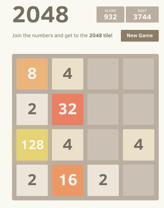
The basic premise is you keep combining similarly numbered blocks to get higher and higher numbered blocks. To win the game, you get the coveted 2048 block. I know our own Linux Journal bookkeeper has gotten further than that, however, and has scored at least 4096, with rumors of getting as high as 8192. Do you like math? Do you hate sleep? This game might be just for you. And like the title says, I'm so, so sorry. Get your copy today—just search for “2048” at the Google Play store. (There are several similar games, I don't want to favor one over the other.)
If you don't want to play on your phone, you can play on-line at gabrielecirulli.github.io/2048.
Occasionally as seasoned Linux users, we run across simple things we never knew existed—and are amazed. Whether it's tab autocompletion, sudo !! for when you forgot to type sudo or even recursive file listing with ls, the smallest tricks can be so incredibly useful. Not long ago, I had one of those moments.
Most people know rc.local is the file where you put commands you want to have start on system boot. Sometimes the rc.local script is disabled, however, and it doesn't work. It also can be difficult to remember the syntax for starting a particular program as a specific user. Plus, having a long list of programs in rc.local can just become ugly. Little did I know, cron supports not only periodic execution of commands, but it also can start programs when the system starts as well!
A normal crontab entry looks like this:
* * * * * /usr/bin/command
That runs the command every minute. There are countless variations to get very specific intervals, but until recently, I didn't know there were options to the five fields. The following is a crontab entry that runs a command every hour on the hour:
@hourly /usr/bin/command
And, there are many more: @annually, @monthly, @daily, @midnight and most interesting for this article, @reboot. If you have a crontab entry like this:
@reboot /usr/bin/command
it will execute when the system starts up, with the ownership and permission of the person owning the crontab! I researched a lot to make sure it wasn't just on reboot, but also on a cold boot—and yes, the @reboot terminology just means it runs once when the system first boots. I've been using this as a quick hack to start programs, and it works amazingly well.

I know 99.9% of you already knew this juicy bit of info, but for that .1% who have been living in the dark like me, I present you with a sharp new arrow for your system administrator quiver. It's a very simple trick, but all the best ones are!
Portable apps aren't anything new. There are variations of “single executable apps” for most platforms, and some people swear by keeping their own applications with them for use when away from home. I don't usually do that, as most of what I do is on-line, but there is one exception: security.
When I'm asked to help a Windows user figure out what is wrong with his or her computer, I generally take a USB drive and nothing else. I also usually run dd on that Flash drive when I get back home, because Windows can be a breeding ground for nasty infections. In order to build a USB device quickly that I can use to help my Windows friends, I like to use the awesome open-source program at portableapps.com.
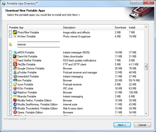
The downloadable program provides a sort of “app store” for downloading individual portable apps. It makes sure all of your apps are up to date, and it's a great way to browse the different categories and look for apps that might be useful. Granted, many of the portable apps themselves aren't open source, but the program that manages them for you is. If you ever need to help friends or acquaintances with their infected systems, a USB drive prepped with the Windows-based portableapps.com application is a great way to start.
In my last few articles, I looked at several different Python modules that are useful for doing computations. But, what tools are available to help you analyze the results from those computations? Although you could do some statistical analysis, sometimes the best tool is a graphical representation of the results. The human mind is extremely good at spotting patterns and seeing trends in visual information. To this end, the standard Python module for this type of work is matplotlib (matplotlib.org). With matplotlib, you can create complex graphics of your data to help you discover relations.
You always can install matplotlib from source; however, it's easier to install it from your distribution's package manager. For example, in Debian-based distributions, you would install it with this:
sudo apt-get install python-matplotlib
The python-matplotlib-doc package also includes extra documentation for matplotlib.
Like other large Python modules, matplotlib is broken down into several sub-modules. Let's start with pyplot. This sub-module contains most of the functions you will want to use to graph your data. Because of the long names involved, you likely will want to import it as something shorter. In the following examples, I'm using:
import matplotlib.pyplot as plt
The underlying design of matplotlib is modeled on the graphics module for the R statistical software package. The graphical functions are broken down into two broad categories: high-level functions and low-level functions. These functions don't work directly with your screen. All of the graphic generation and manipulation happens via an abstract graphical display device. This means the functions behave the same way, and all of the display details are handled by the graphics device. These graphics devices may represent display screens, printers or even file storage formats. The general work flow is to do all of your drawing in memory on the abstract graphics device. You then push the final image out to the physical device in one go.
The simplest example is to plot a series of numbers stored as a list. The code looks like this:
plt.plot([1,2,3,4,3,2,1]) plt.show()
The first command plots the data stored in the given list in a regular scatterplot. If you have a single list of values, they are assumed to be the y-values, with the list index giving the x-values. Because you did not set up a specific graphics device, matplotlib assumes a default device mapped to whatever physical display you are using. After executing the first line, you won't see anything on your display. To see something, you need to execute the second show() command. This pushes the graphics data out to the physical display (Figure 1). You should notice that there are several control buttons along the bottom of the window, allowing you to do things like save the image to a file. You also will notice that the graph you generated is rather plain. You can add labels with these commands:
plt.xlabel('Index')
plt.ylabel('Power Level')
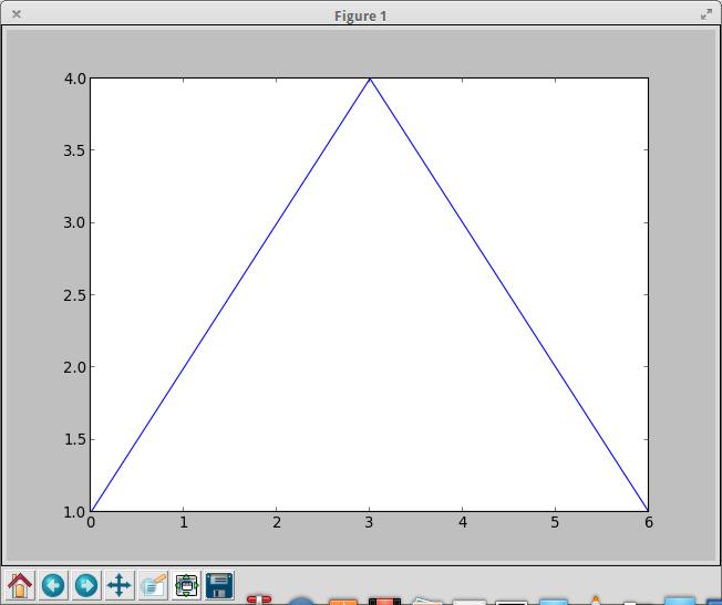
Figure 1. A basic scatterplot window includes controls on the bottom of the pane.
You then get a graph with a bit more context (Figure 2). You can add a title for your plot with the title() command, and the plot command is even more versatile than that. You can change the plot graphic being used, along with the color. For example, you can make green triangles by adding g^ or blue circles with bo. If you want more than one plot in a single window, you simply add them as extra options to plot(). So, you could plot squares and cubes on the same plot with something like this:
t = [1.0,2.0,3.0,4.0]
plt.plot(t,[1.0,4.0,9.0,16.0],'bo',t,[1.0,8.0,27.0,64.0],'sr')
plt.show()
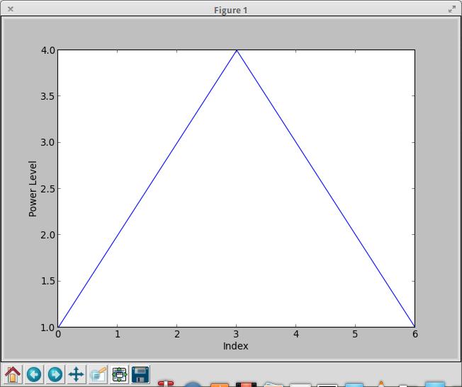
Figure 2. You can add labels with the xlabel and ylabel functions.
Now you should see both sets of data in the new plot window (Figure 3). If you import the numpy module and use arrays, you can simplify the plot command to:
plt.plot(t,t**2,'bo',t,t**3,'sr')
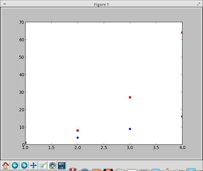
Figure 3. You can draw multiple plots with a single command.
What if you want to add some more information to your plot, maybe a text box? You can do that with the text() command, and you can set the location for your text box, along with its contents. For example, you could use:
plt.text(3,3,'This is my plot')
This will put a text area at x=3, y=3. A specialized form of text box is an annotation. This is a text box linked to a specific point of data. You can define the location of the text box with the xytext parameter and the location of the point of interest with the xy parameter. You even can set the details of the arrow connecting the two with the arrowprops parameter. An example may look like this:
plt.annotate('Max value', xy=(2, 1), xytext=(3, 1.5),
 ↪arrowprops=dict(facecolor='black', shrink=0.05),)
Several other high-level plotting commands are available. The bar() command lets you draw a barplot of your data. You can change the width, height and colors with various input parameters. You even can add in error bars with the xerr and yerr parameters. Similarly, you can draw a horizontal bar plot with the barh() command. Or, you can draw box and whisker plots with the boxplot() command. You can create plain contour plots with the contour() command. If you want filled-in contour plots, use contourf(). The hist() command will draw a histogram, with options to control items like the bin size. There is even a command called xkcd() that sets a number of parameters so all of the subsequent drawings will be in the same style as the xkcd comics.
Sometimes, you may want to be able to interact with your graphics. matplotlib needs to interact with several different toolkits, like GTK or Qt. But, you don't want to have to write code for every possible toolkit. The pyplot sub-module includes the ability to add event handlers in a GUI-agnostic way. The FigureCanvasBase class contains a function called mpl_connect(), which you can use to connect some callback function to an event. For example, say you have a function called onClick(). You can attach it to the button press event with this command:
fig = plt.figure()
...
cid = fig.canvas.mpl_connect('button_press_event', onClick)
Now when your plot gets a mouse click, it will fire your callback function. It returns a connection ID, stored in the variable cid in this example, that you can use to work with this callback function. When you are done with the interaction, disconnect the callback function with:
fig.canvas.mpl_disconnect(cid)
If you just need to do basic interaction, you can use the ginput() command. It will listen for a set amount of time and return a list of all of the clicks that happen on your plot. You then can process those clicks and do some kind of interactive work.
The last thing I want to cover here is animation. matplotlib includes a sub-module called animation that provides all the functionality that you need to generate MPEG videos of your data. These movies can be made up of frames of various file formats, including PNG, JPEG or TIFF. There is a base class, called Animation, that you can subclass and add extra functionality. If you aren't interested in doing too much work, there are included subclasses. One of them, FuncAnimation, can generate an animation by repeatedly applying a given function and generating the frames of your animation. Several other low-level functions are available to control creating, encoding and writing movie files. You should have all the control you require to generate any movie files you may need.
Now that you have matplotlib under your belt, you can generate some really stunning visuals for your latest paper. Also, you will be able to find new and interesting relationships by graphing them. So, go check your data and see what might be hidden there.
When I wrote about Usenet and Sickbeard a while back, I got many e-mails that I had broken the first rule of Usenet: don't talk about Usenet. I'm a sucker for freedom though, and I can't help but share when cool programs are available. This month, I switched from Sickbeard to NZBDrone for managing my television shows.
NZBDrone is a program designed to manage a local collection of television shows. It also has the capability of working with Usenet programs to automate the possibly illegal downloading of episodes, but that's truly not all it's good for. NZBDrone will take your TV show files and organize them into folders, download metadata and let you know if you're missing files. It also will show you when your favorite shows are going to be airing next.
Although it hasn't given me a problem, the fact that NZBDrone runs on Mono makes me nervous. The installation guide on the www.nzbdrone.com Web site makes setup simple enough, but there will be a boatload of dependencies that you might have to install due to its Mono infrastructure.
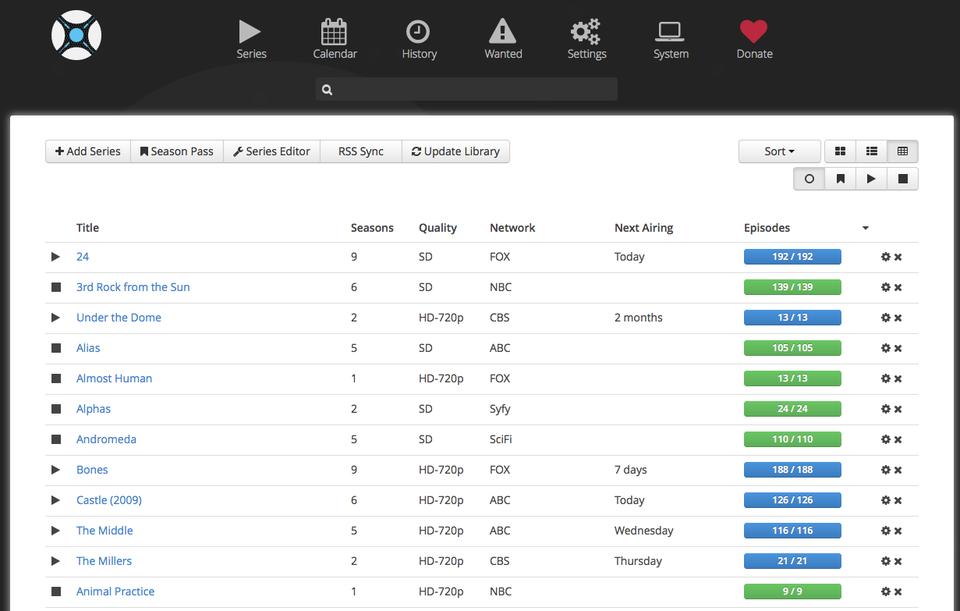
NZBDrone will work with your existing Plex media server, XBMC machines and SABNzb installs, and it automatically performs most of its features if you allow it to do so. The interface is beautiful, and even with a large collection of television shows (I have more than 15TB of TV shows on my server), it's very responsive. Whether you record your TV episodes, rip your television season DVDs or find your episodes in other ways, NZBDrone is a perfect way to manage your collection. It's so intuitive and user-friendly, that it gets this month's Editors' Choice award!
Work and acquire, and thou hast chained the wheel of Chance.
—Ralph Waldo Emerson
Our lives begin to end the day we become silent about things that matter.
—Martin Luther King Jr.
Millions long for immortality who don't know what to do with themselves on a rainy Sunday afternoon.
—Susan Ertz
People laugh at me because I use big words. But if you have big ideas you have to use big words to express them, haven't you?
—L. M. Montgomery
Our patience will achieve more than our force.
—Edmund Burke