
By Marcus Nasarek
In the past 15 years, hard disk capacities have grown by a factor of almost a thousand. 15 years ago, a typical hard disk had a capacity of between 300 and 500 Mbytes, and they were just as expensive as today's 300 to 500 Gbyte disks. Because PCs with two or more disks are now quite common, home users can easily afford the data redundancy and higher performance that used to be the reserve of enterprise-level servers. The technology that makes this possible is known as RAID.
RAID [1] was designed some 20 years ago by Berkeley post-graduate students David Patterson, Garth Gibson, and Randy Katz. At the time, RAID was the answer to a difficult problem: if you needed a lot of storage capacity, you had to choose either a single, large disk that was reliable but expensive or a lot of small, fairly unreliable, inexpensive disks.
One problem with small disks was that the management effort involved in replacing a single large disk with many small disks was too high. RAID was a scheme for addressing a multiple-disk array as a single unit. The proposed solution also addressed the risk of data loss, in case a single disk in the array failed. The paper they published was titled "A Case for Redundant Array of Inexpensive Disks (RAID)." When the price of large disks stopped being an issue some time later, the word Inexpensive was replaced with Independent.
In the simplest RAID scenario, you can group a number of disks to form a single unit, and present that unit to the application layer as a single, logical disk. This is what geeks typically refer to as JBOD ("Just a Bundle of Disks"). But RAID can do far more. RAID serves as a management layer between the filesystem and the hardware that lets you exploit the physical characteristics of the disk array. Various RAID alternatives offer a range of solutions for improving performance or mitigating the risk of disk failure.
The various RAID alternatives are referred to as RAID Levels, although the term level does not imply a hierarchy; instead, the different RAID levels are really completely independent designs. The seven basic RAID levels are known as RAID 0 through RAID 7. See the box titled "RAID Levels" for more on these RAID alternatives.
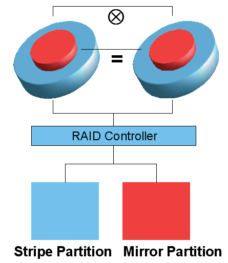
RAID levels 0 and 1 are the most important levels for home use. Level 0 is also known as striping, and gives you best possible performance. Level 1 provides a high level of redundancy and is known as mirroring. For users who can't decide whether they need more performance or more redundancy, there is a special RAID level for home use known as RAID 1.5. However, this level is a trade-off: at least four disks are needed to combine the properties of Level 0 and Level 1. RAID 1.5 combines Levels 0 and 1 using just two disks, and presents the RAID disks separately to the application layer (Figure 1).
| RAID Levels |
|
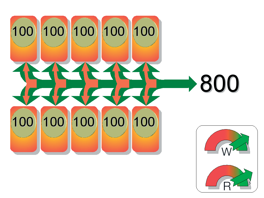
Besides the well-known RAID levels 0 and 1, there are a number of different RAID designs. The original work done by Patterson, Gibson, and Katz covered levels 1 through 5. Levels 0 and 6 were added later, as were various proprietary solutions. RAID levels 2 through 4, 6 and 7 are less popular and have become more or less insignificant. Combinations of the other designs have led to levels known as Level 0+1, 10, 30, 15, 50, 51, 55, and RAID-Z. RAID 0 groups disks and distributes the load evenly over the disks. This greatly improves access speeds. The total capacity of the array is equal to the sum of the capacities of both disks. The risk of failure is quite high as this level offers nothing in the line of redundancy. RAID 1 writes identical data simultaneously to all the disks in the array. The total capacity of the array is equal to the capacity of a single disk. Read access is typically quicker than with a single disk, and write access is about the same speed. RAID 2 was quite common for mainframes in former times, but it is fairly insignificant now. A RAID 2 array needs at least 10 disks. Sophisticated error checking lets users discover both hard disk failures and write errors. Assuming 10 disks, the access time ratio for reading and writing is 1 to 8 compared with a single disk. By adding the hard disk data bitwise, and storing the results, you can restore the data lost when a disk fails by reference to the existing data and the results of the addition. The result of the addition is referred to as the parity. RAID 3 stores the parity data for the array on a single disk. As the parity disk is used much more than the data disks, it has a natural tendency to fail first. RAID 4 represents a minor modification to RAID 3: whereas RAID 3 uses byte striping, RAID 4 processes whole payload data blocks. As a result, RAID 4 can handle small files more effectively, whereas RAID 3 only comes to its own with contiguous files. Just like RAID 3, RAID 4 uses a separate parity disk. RAID 5 is the cheapest version of redundant data storage. Assuming at least three disks in the array, it gives you 66 percent of the gross capacity for payload data in contrast to 50 percent with RAID 1. The more disks you add, the better the numbers become. RAID 5 distributes data and parity information evenly over all the disks in the array, meaning that the disks are subject to about the same levels of wear and tear. On the downside, rebuilding the RAID following a disk failure takes much longer than with RAID 1. Depending on your application, you can combine the basic RAID levels more or less arbitrarily. RAID 10 implements a RAID 0 array using two RAID 1 arrays. RAID 1 provides redundancy for more data security, while RAID 0 adds performance. It you have at least six disks, a combination of RAID 5 and 0 (RAID 50) is even more efficient. |
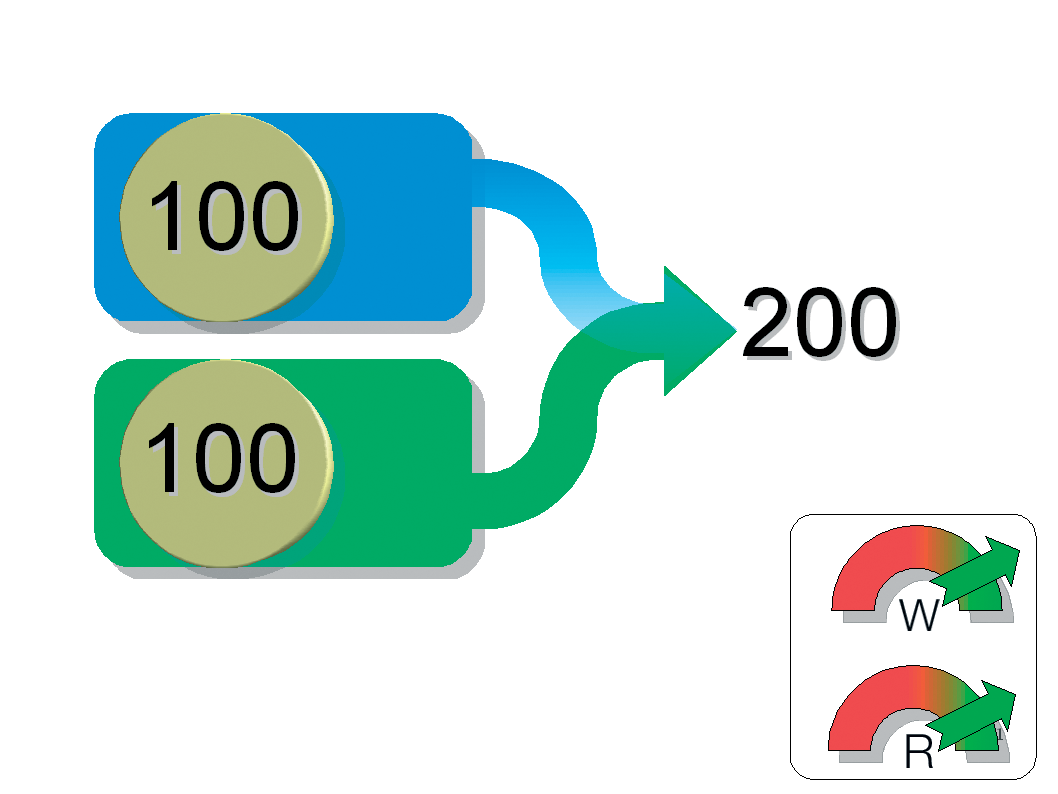

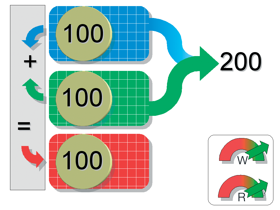
Striping (RAID 0) involves stringing disks together and addressing them blockwise (in "stripes). When an application needs to write data, the RAID controller distributes the load over all the disks.
From a technical point of view, the controller simply dumps the data into the hard disk cache and goes straight to the next disk. By the time the controller talks to the first disk again, the disk will have had enough time to finish the task and should have the results ready for the controller to pick up. If you use two disks, access times should theoretically be twice as fast.
Of course, RAID 0 does not distribute data character-wise; instead, it uses data blocks with a certain striping granularity. The probability of a failure increases the more disks you add to the array. Thus, striping is recommended for systems where speed is far more important than redundancy.
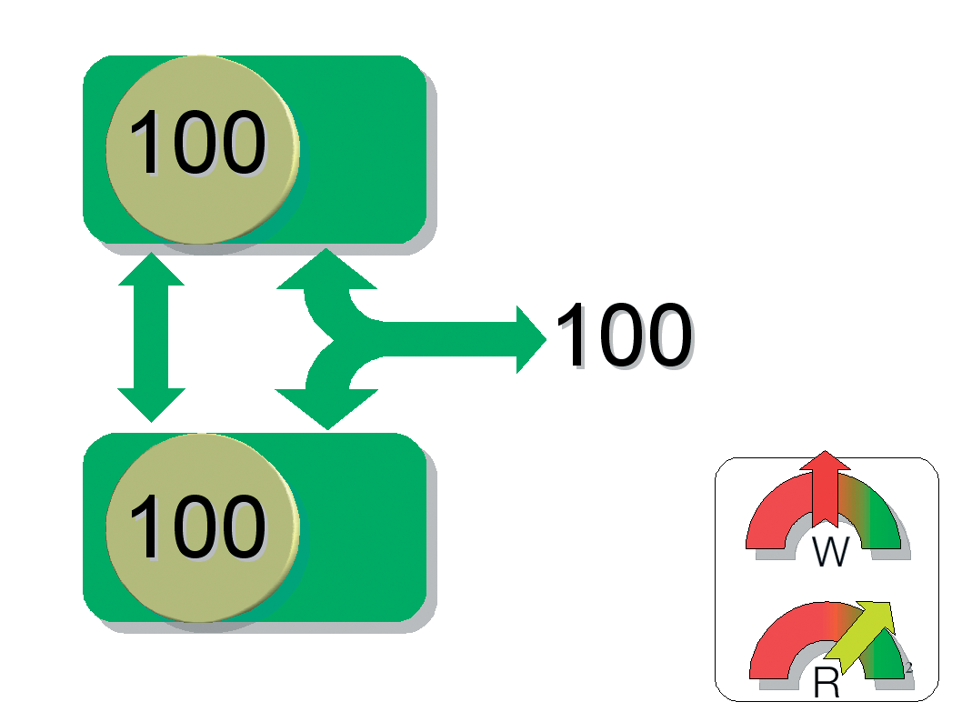
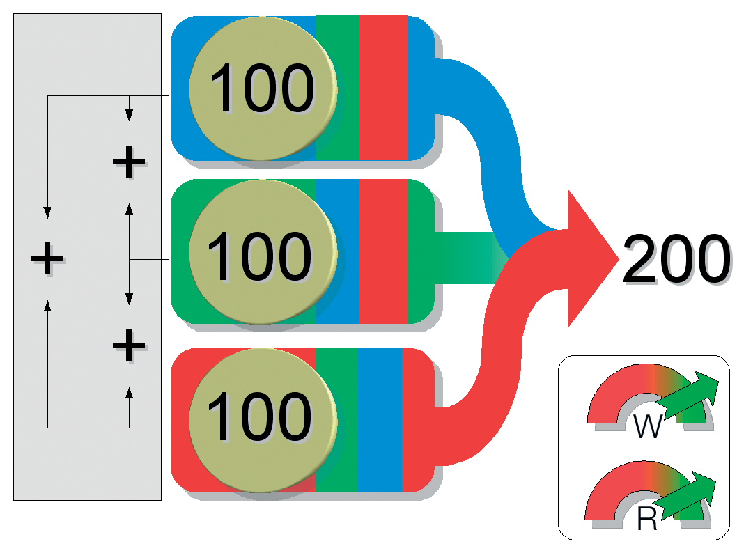
Mirroring (RAID 1) is exactly the opposite to striping. It addresses the disks in series and writes the data to each disk in the array; in other words, RAID 1 mirrors the data. However, storing identical copies of the data on each hard disk means that the total capacity of the array is no bigger than that of a single disk. If you use two 200GByte disks, the net capacity is just 200GBytes rather than 400. While the write access time is no different from the time for a single disk, read access is much quicker, as the controller can read from both disks in parallel.
The big advantage that RAID 1 offers is that, if one disk fails, the data is still available on the other disk. However, this only applies to physical defects: logical errors, such as inadvertent deleting, modifying, or overwriting of files on the filesystem, are mirrored to the other disk in realtime. In other words, RAID 1 does not protect you against human error or software failures.
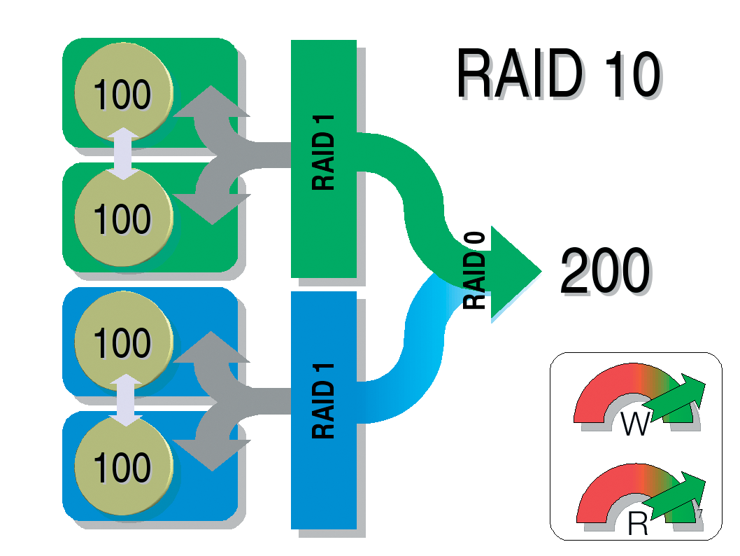
To leverage the benefits of RAID levels 0 and 1 at the same time, you need a PC with at least four disks for a combined RAID 10 approach (see the "RAID Level Overview" box) - this is not an option for most users. Some vendors are aware that most desktop users don't want to use four disks and offer an elegant compromise that uses just two disks.
RAID 1.5, as this approach is known, divides each of the two disks into two areas. The controller combines one of these areas on each of the disks to provide a RAID 1 array, while combining the other two areas to provide a RAID 0 array. This approach is shown on the right of Figure 1.
DFI and EPox were the first motherboard manufacturers to introduce this RAID variant, however, the vendors failed to come up with the goods; both boards just built RAID 1 arrays. The performance benefits were drawn from faster reading speeds. Finally, Intel came up with the ICH6R I/O controller for the new Serial ATA disks to introduce "Intel Matrix RAID", which provides genuine RAID 1.5 support.
The various RAID designs were originally implemented as software solutions. As the computational effort of a software-only approach proved to be too much for CPUs at the time, it was not long until the first RAID controller cards were introduced to provide a more powerful, hardware-based approach. This kind of implementation is known as hardware RAID.
The more powerful CPUs became, the easier it was to implement software-only RAID. Low-budget software RAID became common on home machines running Linux. Software RAID arrays are typically not as fast as their hardware-based counterparts. The load on the CPU is normally very noticeable in everyday operations. Benefits such as parallel access are difficult to exploit with software-only drivers.
RAID became more popular with home users when board vendors started adding RAID controller chips to their hardware. Today, most modern boards, especially the ones with connectors for fast S-ATA disks, have some kind of RAID support. The integrated chips on most motherboards only handle part of the management, leaving the drivers the lion's share of the work. And getting this to work is not always trivial.
Software-based RAID was introduced to Linux a long time ago. Computers now have enough power to handle the additional load of managing an array of disks almost transparently, and the performance benefit from a motherboard-based solution can be marginal, as it relies to a great extent on software drivers.
For your first steps with RAID, it is perfectly okay to install a software-based variant. To do so, you will need root privileges on the machine in question, along with at least two free partitions and the Mdadm tool ([2]). Make sure the partitions are free of data, as we will be deleting the filesystems on these partitions in the course of our experiments.
You could even use a USB stick for your first RAID experiments; you will need to partition the stick with a tool such as Gparted, Qtparted, or Cfdisk. The experiment involves the following steps:
The following example uses a USB device referred to as /dev/sdc and two partitions referred to as /dev/sdc1 and /dev/sdc2. To build a RAID 1 array, give the following mdadm command:
mdadm --create --verbose /dev/md0 --level=1
-raid-devices=2 /dev/sdc1 /dev/sdc2
The --create option creates the RAID; --verbose gives you more detailed progress information; /dev/md0 is the name of the resulting RAID device, and --level=1 sets the level of redundancy to RAID level 1. The last parameter passes in the number of RAID partitions and their names.
Before you can use the newly created RAID array, you first need to format it (using ReiserFS in our example) and to mount the resulting filesystem:
mkreiserfs /dev/md0
mkdir /media/RAID
mount /dev/md0 /media/RAID
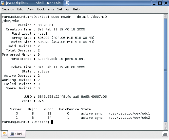
Now you can use the /media/RAID directory like any normal drive. However, in the background, your data will be written to two partitions to provide redundancy. The mdadm --detail /dev/md0 command gives you information on the RAID array status. Figure 2 shows the output from this command.
RAID offers a number of benefits for home users. You achieve more data redundancy and faster disk access with RAID. The Mdadm tool will help you implement any of the RAID levels introduced in this article.
| INFO |
|
[1] RAID on Wikipedia: http://en.wikipedia.org/wiki/RAID
[2] Mdadm: http://cgi.cse.unsw.edu.au/~neilb/mdadm |