By Neil J. Gunther
Most Linux system administrators are familiar with those three little numbers that appear in shell commands like procinfo, uptime, top, and remote host ruptime. Uptime, for example, emits:
9:40am up 9 days, load average: 0.02, 0.01, 0.00
The load average metrics are always included within the output of commands like uptime. While the load average is well known to Linux system administrators, its meaning is often poorly understood. The man page for uptime states that these values represent
a one line display of ... the system load averages for the past 1, 5, and 15 minutes.
which explains why there are three numbers, but it does not explain what the word load means or how to use these figures to forecast and troubleshoot system performance. This article takes a close look at the load average metrics and how to use them.
I'll start with a small experiment to demonstrate how the load average values respond to changes in system load. Experimental load averages were sampled over a one-hour period (3600 seconds) on an otherwise quiescent single-CPU Linux box. These tests consisted of two phases. Two CPU-intensive jobs were initiated as background processes and allowed to execute for 2100 seconds.At that point, these two processes were stopped simultaneously, but load average measurements were continued for another 1500 seconds after the jobs stopped.
Listing 1 is a Perl script that was used to sample the load average every 5 seconds using the uptime command
| Listing 1: Sampling the load average |
01 #! /usr/bin/perl -w
02 $sample_interval = 5; # seconds
03
04 # Fire up background cpu-intensive tasks ...
05 system("./burncpu &");
06 system("./burncpu &");
07
08 # Perpetually monitor the load average via uptime
09 # and emit it as tab-separated fields for possible
10 # use in a spreadsheet program.
11 while (1) {
12
13 @uptime = split (/ /, 'uptime');
14 foreach $up (@uptime) {
15 # collect the timestamp
16 if ($up =~ m/(\d\d:\d\d:\d\d)/) {
17 print "$1\t";
18 }
19 # collect the three load metrics
20 if ($up =~ m/(\d{1,}\.\d\d)/) {
21 print "$1\t";
22 }
23 }
24 print "\n";
25 sleep ($sample_interval); }
|
A C program called burncpu.c was designed to waste CPU cycles. Output from top shows the two instances of burncpu ranked as the highest CPU consumers during the measurement period when getload was running (Table 1).
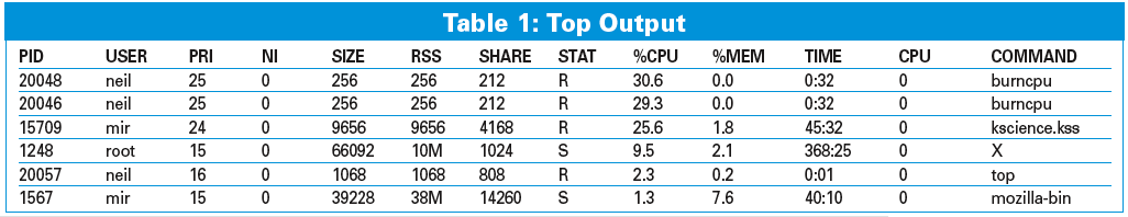
Figure 1 shows that the 1-minute load average reaches a value of 2.0 after 300 seconds into the test; the 5-minute load average reaches 2.0 at around 1200 seconds; the 15-minute load average would reach 2.0 at approximately 4500 seconds; but the processes were killed at 2100 seconds.
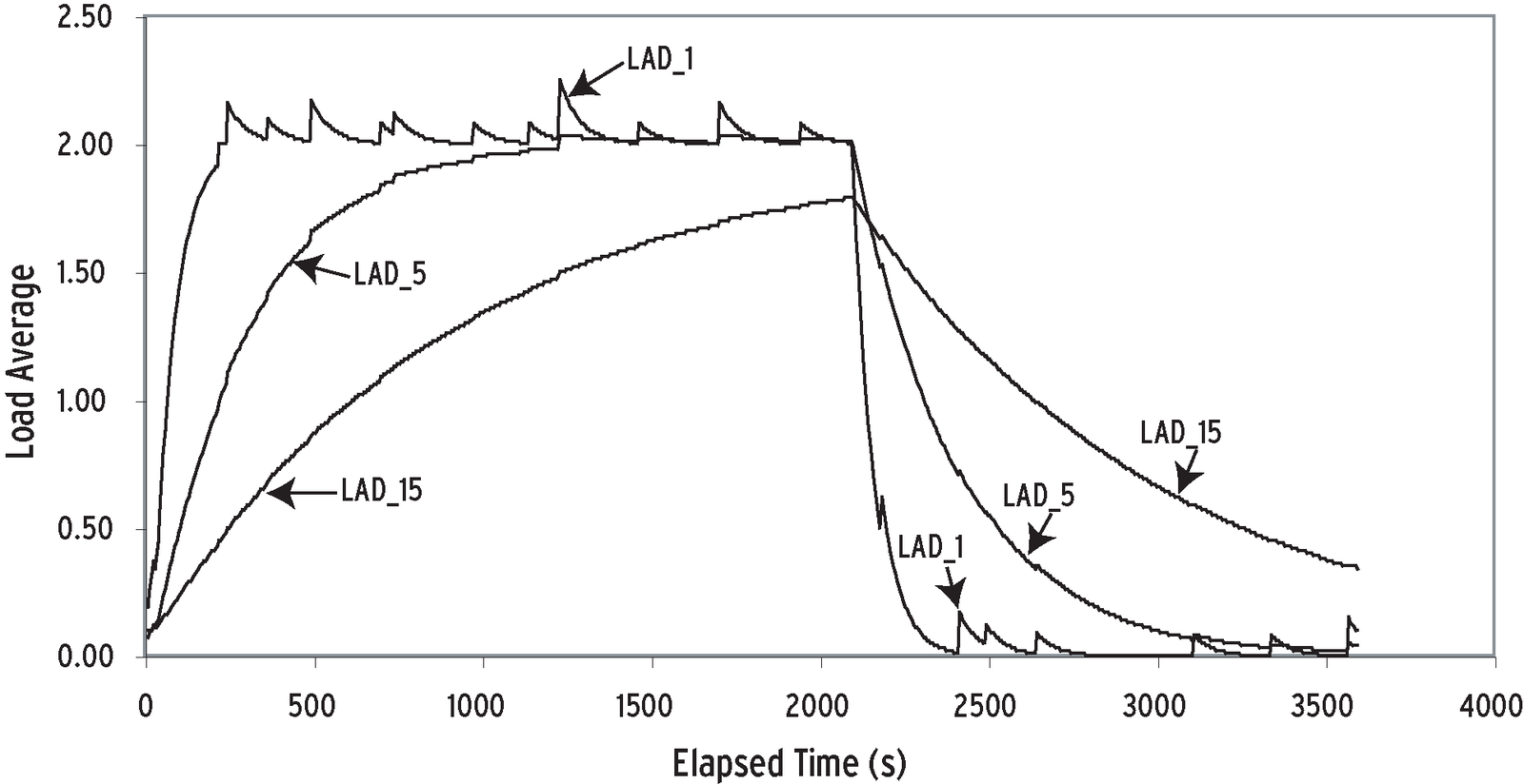
Readers with a background in electrical engineering will immediately spot the striking resemblance between the data in Figure 1 and the voltage curves produced by charging and discharging an RC circuit. Notice that the maximum load during the test is equivalent to the number of CPU-intensive processes running at the time of the measurements. The "fins" in the top curve are a result of various daemons waking up temporarily and then going back to sleep.
My next objective was to explain why the load average data from these experiments exhibits the characteristics seen in Figure 1. For that, I needed to explore the Linux kernel code that calculates the load average. I chose to use the Linux 2.6.20.1 source code [1], complete with cross-referencing hyperlinks for easier navigation and enhanced readability.
Looking at the source code for the CPU scheduler [2], we find the C function function shown in Listing 2. This is the primary routine that calculates the load average metrics. Essentially, the routine checks to see whether the sample period has expired, resets the sampling counter, and calls the subroutine CALC_LOAD to calculate each of the 1-minute, 5-minute, and 15-minute metrics. The sampling interval used for LOAD_FREQ is 5*HZ. How long is that interval?
| Listing 2: calc_load |
01 1136 unsigned long avenrun[3];
02 1137
03 1138 EXPORT_SYMBOL(avenrun);
04 1139
05 1140 /*
06 1141 * calc_load -given tick count, update the avenrun load estimates.
07 1142 * This is called while holding a write_lock on xtime_lock.
08 1143 */
09 1144 static inline void calc_load(unsigned long ticks)
10 1145 {
11 1146 unsigned long active_tasks; /* fixed-point */
12 1147 static int count = LOAD_FREQ;
13 1148
14 1149 count -= ticks;
15 1150 if (unlikely(count < 0)) {
16 1151 active_tasks = count_active_tasks();
17 1152 do {
18 1153 CALC_LOAD(avenrun[0], EXP_1, active_tasks);
19 1154 CALC_LOAD(avenrun[1], EXP_5, active_tasks);
20 1155 CALC_LOAD(avenrun[2], EXP_15, active_tasks);
21 1156 count += LOAD_FREQ;
22 1157 } while (count < 0);
23 1158 }
24 1159 }
|
Every Linux platform has a clock implemented in hardware. This hardware clock has a constant ticking rate by which the system is synchronized. To make this ticking rate known, the clock sends an interrupt to the kernel on every clock tick. The actual interval between ticks differs. Most Linux systems have the CPU tick interval set to 10ms of wall-clock time.
The specific definition of the tick rate is contained in a constant labeled HZ that is maintained in a system-specific header file called param.h. For the online Linux source code we are using here, you can see the value is 100 for an Intel platform in lxr.linux.no/source/include/asm-i386/ param.h, and for a SPARC-based system in lxr.linux.no/source/include/asm-sparc/param.h.
calc_load is called at a frequency defined by the tick rate - once every 5 seconds (not 5 times per second, as some people think). This sampling period of 5 seconds is independent of the 1-, 5-, and 15-minute reporting periods.
The calc_load function in Listing 2 refers to the C macro CALC_LOAD, which does the real work of calculating the load average (Listing 3). CALC_LOAD is defined in http://lxr.linux.no/source/include/linux/sched.h.
| Listing 3: CALC_LOAD() |
98 /* 99 * These are the constant used to fake the fixed-point load-average 100 * counting. Some notes: 101 * - 11 bit fractions expand to 22 bits by the multiplies: this gives 102 * a load-average precision of 10 bits integer + 11 bits fractional 103 * - if you want to count load-averages more often, you need more 104 * precision, or rounding will get you. With 2-second counting freq, 105 * the EXP_n values would be 1981, 2034 and 2043 if still using only 106 * 11 bit fractions. 107 */ 108 extern unsigned long avenrun[]; /* Load averages */ 109 110 #define FSHIFT 11 /* nr of bits of precision */ 111 #define FIXED_1 (1<<FSHIFT) /* 1.0 as fixed-point */ 112 #define LOAD_FREQ (5*HZ) /* 5 sec intervals */ 113 #define EXP_1 1884 /* 1/exp(5sec/1min) as fixed-point */ 114 #define EXP_5 2014 /* 1/exp(5sec/5min) */ 115 #define EXP_15 2037 /* 1/exp(5sec/15min) */ 116 117 #define CALC_LOAD(load,exp,n) \ 118 load *= exp; \ 119 load += n*(FIXED_1-exp); \ 120 load >>= FSHIFT; |
Mathematically, CALC_LOAD is equivalent to taking the current value of the variable load and multiplying it by a factor called exp. This value of load is then added to a term comprising the number of active processes n multiplied by another variable called FIXED_1-exp. The last line of the macro decimalizes the value of load.
We also know that the macro variable exp is equivalent to e-sigma/r (see the box on "Fixed-Point Arithmetic"), and FIXED_1-exp is equivalent to 1 - e-sigma/r. Writing the CALC_LOAD macro in more conventional mathematical notation produces:
![]()
where L(t) is the current value of the load variable, L(t - 1) is its value from the previous sample, and n(t) is the number of currently active processes.
A Linux process can be in one of about half a dozen states (depending on how you count), of which running, runnable (R in the ps command), and sleeping (S in ps command) are the three primary states. Each load-average metric is based on the total number of processes that are:
In queueing theory terminology, the total active processes is called a queue. It literally means not just those processes that are in the waiting line (the so-called run queue), but also those that are currently being serviced (i.e., running). So, CALC_LOAD is the fixed-point arithmetic version of equation (1). (See the box titled "Fixed-Point Arithmetic.")
| Fixed-Point Arithmetic |
|
The cryptic comment that precedes the CALC_LOAD macro in Listing 3 alerts us to the fact that fixed-point, rather than floating-point, arithmetic is used to calculate the load average. A fixed-point representation means that only a fixed number of digits, either decimal or binary, are used to express any number, including those that have a fractional part (mantissa) following the decimal point. Suppose, for example, that 4 bits of precision were allowed in the mantissa. You could precisely represent: 0.1234, -12.3401, 1.2000, 1234.0001 However, numbers like: 0.12346, -8.34051 could not be represented exactly and would be rounded off. Too much rounding can cause insignificant errors to compound into significant errors. One way around this is to increase the number of bits used to express the mantissa, assuming enough storage is available to accommodate the greater precision. Suppose 10 bits are allowed for the integer part and 11 bits for the factional part. This is called an M.N = 10.11 format. The rules for fixed-point addition are the same as for integer addition; however, an important difference occurs with fixed-point multiplication. The product of two M.N fixed-point numbers is:
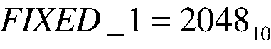
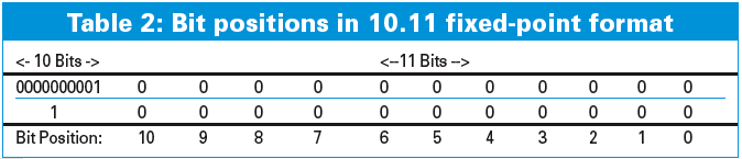
To get back to M.N format, the lower order bits are eliminated by shifting N bits. CALC_LOAD uses serveral fixed-point constants. The first is the number 1, which is labeled FIXED_1. In Table 2, the top row corresponds to FIXED_1 expressed in 10.11 format, whereas the leading zeros and the decimal point have been dropped in the second row. The digits of the resulting binary 1000000000002 are indexed 0 through 11 on the last row of Table 2. This establishes that FIXED_1 is equivalent to 2 to the11th power, or decimal 2048. Using the C left-shift bitwise operator (<<), 1000000000002 can be written as 1 << 11, which is in agreement with line 111 of the macro code. Alternatively, we can write FIXED_1 as a decimal integer:
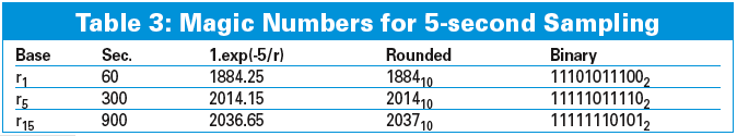
to simplify calculation of the remaining constants: EXP_1, EXP_5, and EXP_15, for the 1-, 5-, and 15-minute metrics. Consider the 1-minute metric as an example. If we denote the sample period as s and the reporting period as r :
sigma = 5 seconds and for the 1-minute metric and r = 60 seconds. Furthermore, the decimal value of EXP_1 is:
To convert this to a 10.11 fixed-point fraction, you only need to multiply it by the fixed-point constant FIXED_1 or 1 to produce:
and round it to the nearest 11-bit integer. Each of the other magic numbers can be calculated in the same way, and the results are summarized in Table 3. The results in Table 3 agree with the kernel defines: #define EXP_1 1884 #define EXP_5 2014 #define EXP_15 2037 |
It turns out that there is nothing particularly novel about the way the load average is calculated. In fact, a common technique for processing highly variable raw data for subsequent analysis is to apply some kind of smoothing function to that data. The general relationship between the raw input data and the smoothed output data is given by:
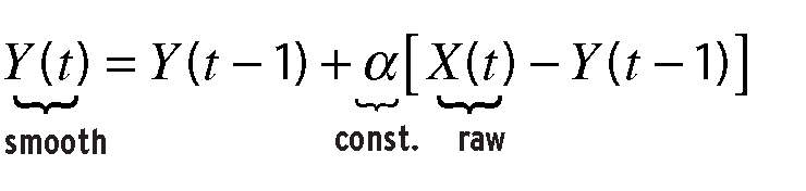
The smoothing function in equation (2) is an exponential filter or exponentially smoothed moving average of the type used in financial forecasting [3] and signal processing. The parameter a in equation (2) is commonly called the smoothing constant, while (1 - a) is called the damping factor. Both these factors can be directly related to the corresponding factors in equation (1). The magnitude of the smoothing coefficient (0 <= a <= 1) determines how much the current forecast must be corrected for error in the previous iteration of the forecast.
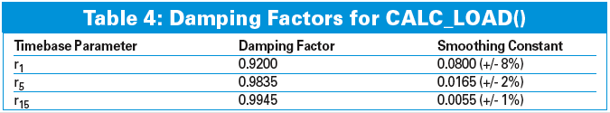
Notice that the exponential damping factor for r1 in Table 4 agrees with the value calculated in the "Fixed-Point Arithmetic" sidebar to four decimal places. The 1-minute load average metric has the least damping, or about 8% correction, because it is the most responsive to instantaneous changes in the length of the run queue. Conversely, the 15-minute load average has the most damping, or only 1% correction, because it is the least responsive metric.
Inevitably, the question arises: What is a good load average? Since we now know that the load average is an exponentially damped moving average of activity in the process run queue, we could convert the question to, "How long should my queue be?"
Long queues correspond to long response times, so it's really the response time metric that should get your attention. One consequence is that a long queue can cause "poor response times," but that depends on what poor means. In most performance management tools, there is a disconnect between the measured run-queue length and the user-perceived response times. Another problem is that queue length is an absolute measure, whereas what is really needed is a relative performance measure. Even the words poor and good are relative terms. Such a relative metric is called the stretch factor, and it measures the mean queue length relative to the mean number of requests already in service. It is expressed in multiples of service units. A stretch factor of 1 means no waiting time is involved.
What makes the stretch factor really useful is that it can easily be compared with service level targets. Service targets are usually expressed in certain types of business units (e.g., quotes per hour is a common business unit of work for an insurance industry). The expected service level is called the service level objective or SLO, and it is expressed as multiples of the relevant service unit. An SLO might be documented as, "The average user response time is not to exceed 15 service units between the peak operating hours of 10am and 2pm."
This is the same as saying the SLO shall not exceed a stretch factor of 15.
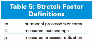
Using the symbols defined in Table 5, the stretch factor f can be calculated as the ratio:
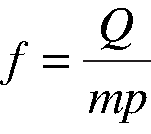
From the experiments described earlier, we know that m = 1 because it was a single-process box, Q = 2 for the 1-minute load average, and p = 1 because the workload was CPU-bound. Substituting these values into equation (3) gives a stretch factor of f = 2. This result tells us that the expected time for any process to complete is two service periods. Notice that we don't have to know what the actual service period is. The stretch factor and the load average happen to be identical in this case, because the processes are running on a single processor and they are CPU-intensive. I'll describe a couple scenarios for using this stretch factor in real situations.
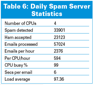
All major email hosting services run spam analyzers. A typical configuration might consist of a set of specialized servers, each raking over email text using a filtering tool like SpamAssassin [4]. One such well-known, and therefore heavily trafficked, web portal has a battery of some 100 servers, each comprising two dual-cores, all performing 24/7 email scanning. Typical daily spam-filtering statistics are shown in Table 6.
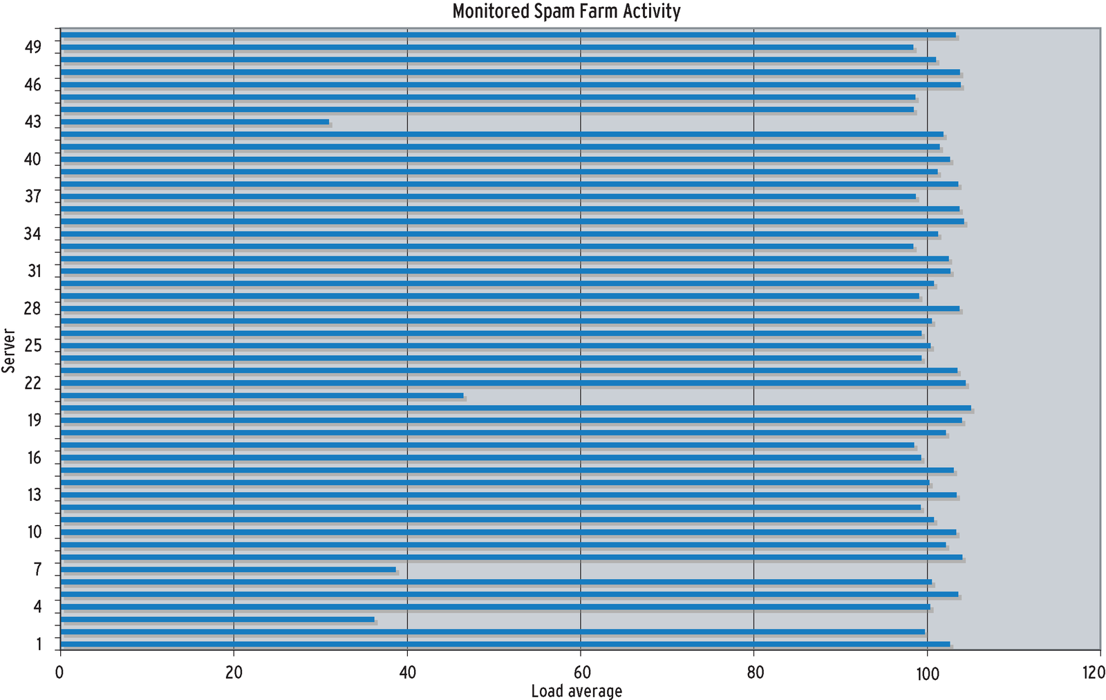
A load balancer was used to distribute work into the server farm. The effectiveness of the load balancer was monitored using 1-minute load averages. The sample of these load averages from 50 of the servers (as shown in Figure 2) reveals an imbalance of work in the farm.
A system administrator might ask:
Let's substitute the load average into equation (3) to calculate the stretch factor:
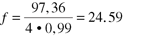
From Table 6, the average time to scan an email message (S) is 6 seconds.
So, a stretch factor of f = 25 service periods implies that it takes about 25 x 6 = 150 seconds or 2.5 minutes from the time an email message reaches the portal until it lands in the intended user's email box.
An absolute value of Q = 97.36 for the load average tells us very little. The relative stretch factor, however, tells you how many service periods the spam filtering is costing.
As for the question about whether a load average of 97.36 is desirable, that depends on the agreed upon service targets. At least now, such questions can be addressed quantitatively instead of speculatively.
You can also use the data in Table 6 to model the performance using a performance-prediction tool like PDQ. (See the box titled "PDQ in Python.")
The spam server model in PyDQ (PDQ in Python) is shown in Listing 4. Running this PDQ model produces a report that contains the output shown in Listing 5.
| Listing 4: PDQ Spam Farm Model |
01 #!/usr/bin/env python import pdq
02 # Measured performance parameters
03 cpusPerServer = 4
04 emailThruput = 2376 # emails per hour
05 scannerTime = 6.0 # seconds per email
06 pdq.Init("Spam Farm Model")
07 # Timebase is SECONDS ...
08 nstreams = pdq.CreateOpen("Email", float(emailThruput)/3600)
09 nnodes = pdq.CreateNode("spamCan", int(cpusPerServer), pdq.MSQ)
10 pdq.SetDemand("spamCan", "Email", scannerTime)
11 pdq.Solve(pdq.CANON)
12 pdq.Report()
|
| Listing 5: PDQ System Performance Output |
01 ****** SYSTEM Performance ******* 02 Metric Value Unit 03 ------ ----- ---- 04 Workload: "Email" 05 Number in system 100.7726 Trans 06 Mean throughput 0.6600 Trans/Sec 07 Response time 152.6858 Sec 08 Stretch factor 25.4476 |
The stretch factor predicted by PDQ is a little bigger than we calculated using equation (3). Why is that? To learn why, you must examine the section of the PDQ report that presents server performance information (Listing 6).
| Listing 6: PDQ Resource Performance Report |
01 ****** RESOURCE Performance ******* 02 Metric Resource Work Value Unit 03 ------ -------- ---- ----- ---- 04 Throughput spamCan Email 0.0660 Trans/Sec 05 Utilization spamCan Email 99.0000 Percent 06 Queue length spamCan Email 100.7726 Trans 07 Waiting line spamCan Email 96.8126 Trans 08 Waiting time spamCan Email 146.6858 Sec 09 Residence time spamCan Email 152.6858 Sec |
Given the rate at which work is arriving (2376 emails per hour), each CPU should be 99% busy. This utilization is higher than seen in the actual spam farm because of the load imbalance. PDQ is assuming ideal load balance across all servers, so more work is getting done. The predicted load average (Queue length metric in the PDQ report) is closer to 100 emails; therefore, the predicted stretch factor of 25.45 is a little larger than the calculated value of 24.59.
Either stretch factor value was considered to be borderline acceptable under peak load conditions. Since all the servers are close to saturated, one recourse is to upgrade with faster CPUs or, more likely, procure new 4-way servers to handle the expected additional work. PDQ helps to size the number of new servers based on current and expected stretch factors. Clearly, it is the stretch factor ratio that provides a more meaningful indicator for performance management than the absolute load average by itself.
| PDQ in Python |
|
PDQ (Pretty Damn Quick) is a modeling tool for analyzing the performance characteristics of computational resources, for example, processors disks and a set of processes that make requests for those resources. A PDQ model is analyzed using algorithms based on queueing theory. The current release facilitates building and analyzing performance models in C, Perl, Python, Java, and PHP. The Python PDQ functions and procedures used in this section are:
PDQ is maintained by Peter Harding and me. You'll find more information about the PDQ library online [5]. |
You can use a similar PyDQ model to see what it means to have no waiting line with all the CPUs busy. In this case, each Linux process takes 10 hours to complete because it is transforming oil-exploration data for further analysis by geophysicists. The corresponding PyDQ model is shown in Listing 7.
| Listing 7: PyDQ Model |
01 #!/usr/bin/env python import pdq
02 processors = 4 # Same as spam farm example
03 arrivalRate = 0.099 # Jobs per hour (very low arrivals)
04 crunchTime = 10.0 # Hours (very long service time)
05
06 pdq.Init("ORCA LA Model")
07 s = pdq.CreateOpen("Crunch", arrivalRate)
08 n = pdq.CreateNode("HPCnode", int(processors), pdq.MSQ)
09 pdq.SetDemand("HPCnode", "Crunch", crunchTime)
10 pdq.SetWUnit("Jobs")
11 pdq.SetTUnit("Hour")
12 pdq.Solve(pdq.CANON)
13 pdq.Report()
|
The PDQ resource performance report corresponding to Listing 7 is in Listing 8. The waiting line is essentially zero length and all four CPUs are busy, though only 25% utilized. If you were to look at the CPU statistics while the system was running, you would observe that each CPU was actually 100% busy. To understand what PDQ is telling us, look at the System Performance section of the PDQ report (Listing 9).
| Listing 8: Resource Performance Output |
01 ****** RESOURCE Performance ******* 02 Metric Resource Work Value Unit 03 ------ -------- ---- ----- ---- 04 Throughput HPCnode Crunch 0.0990 Jobs/Hour 05 Utilization HPCnode Crunch 24.7500 Percent 06 Queue length HPCnode Crunch 0.9965 Jobs 07 Waiting line HPCnode Crunch 0.0065 Jobs 08 Waiting time HPCnode Crunch 0.0656 |
| Listing 9: System Performance Output |
01 ****** SYSTEM Performance ******* 02 Metric Value Unit 03 ------ ----- ---- 04 Workload: "Crunch" 05 Number in system 0.9965 Jobs 06 Mean throughput 0.0990 Jobs/Hour 07 Response time 10.0656 Hour 08 Stretch factor 1.0066 |
The stretch factor is 1 (service period) because there is no waiting line. It takes 10 hours for each job to finish, so the response is about 10 hours.
The reason this appears a little odd is that PDQ makes predictions based on steady-state behavior (i.e., how the system looks in the long run). With a service time of 10 hours, you really need to observe the system for much longer than that to see what it looks like in steady state. Much longer here means on the order of 100 hours or longer. You don't actually need to do that, but PDQ is telling us how things would look if you did.
Since the average service period is relatively large, the request rate is correspondingly small so that no waiting line forms. This, means that the processor utilization of 25% is also low - in the long view. Looking at the system for just a few minutes while it is crunching 10 hours worth of oil-exploration data corresponds to an instantaneous snapshot of the system, not a steady-state view.
Both of the preceding stretch-factor examples involve CPU-bound workloads. I/O-bound workloads (either disk or network) will tend to exhibit smaller load averages than CPU-bound work if those processes become suspended or sleep waiting on data. In that state, they are neither runnable nor running and therefore do not contribute to n(t) in equation (1). Conversely, when the Linux I/O driver is performing work, it runs in kernel mode on a CPU and does contribute to n(t).
The load average value Q measures the total number of requests; both waiting and in service. It is not a very meaningful quantity because it is an absolute value. Combining it, however, with the number of configured processors (m) and their average measured utilization (p), the stretch factor f provides a better performance management metric for symmetric multiprocessor and multicore servers because it is a relative performance indicator that can be compared directly with established SLOs.
The load average provides information about the trend in the growth of the run queue, which is why there are three metrics. Each metric captures trend information from the run queue as it was 1, 5, and 15 minutes ago. Compared with today's graphical data display capabilities, this approach to data representation looks antique. In fact, the load average is one of the earliest forms of operating-system instrumentation (circa 1965).
This article presented the stretch factor as a better way to make use of load average data for managing the performance of application service-level targets on multicore servers.
| INFO |
|
[1] Linux 2.6.20.1 source code: http://lxr.linux.no/source/
[2] Linux scheduler C code: http://lxr.linux.no/source/kernel/timer.c [3] Financial forecasting: http://bigcharts.marketwatch.com [4] SpamAssassin: http://spamassassin.apache.org/ [5] PDQ library: http://www.perfdynamics.com/Tools |
| THE AUTHOR |
|
Neil Gunther, M.Sc., Ph.D. is an internationally recognized consultant who founded Performance Dynamics Company in 1994. Prior to that, Dr. Gunther held research and management positions at San Jose State University, JPL/NASA, Xerox PARC, and Pyramid/Siemens Technology. Performance Dynamics has also embarked on joint research into Quantum Information Technology. Dr. Gunther is a member of the AMS, APS, ACM, CMG, IEEE, and INFORMS. |