By Andreas Romeyke
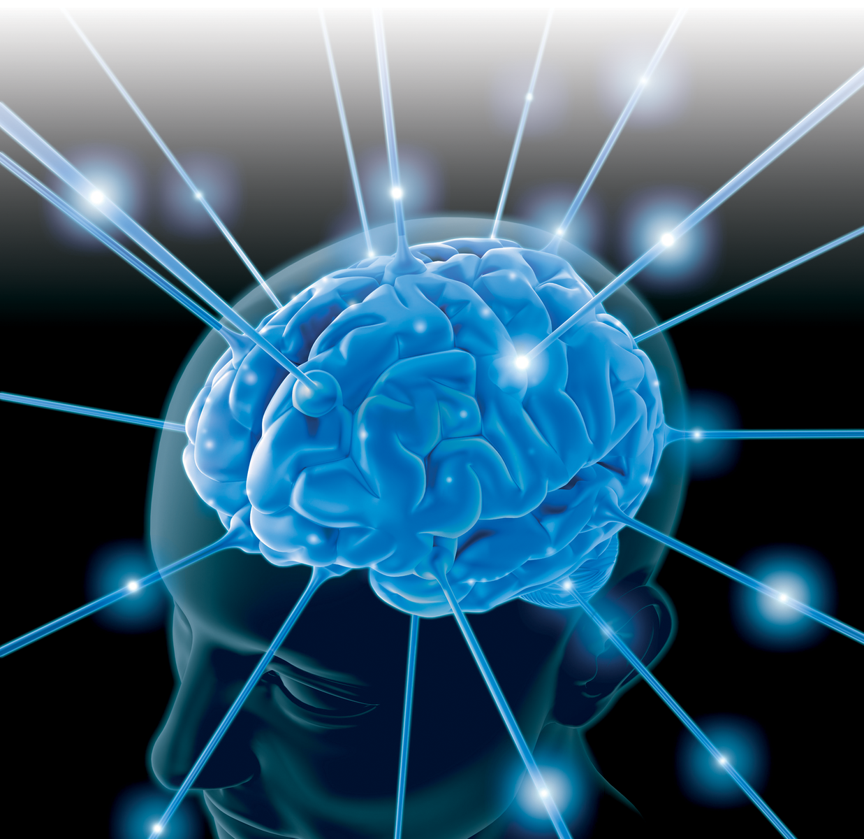
If you look for a route on a map, your eyes will fall fairly directly on an efficient solution. The human brain is capable of making judgments without much attention to optimization algorithms or distance calculations. This intuitive approach is very foreign to digital computers. Conventional computer programs tend to operate through mathematical solutions, which make them inefficient for tasks such as prediction and pattern recognition. An experimental form of program known as an Artificial Neural Network (ANN) addresses this problem by making the computer operate more like a human brain.
An artificial neural network simulates a collection of nerve cells connected by means of weighted paths. One successful use for neural networks is in the field of face recognition. A neural network can recognize a face on the basis of a collection of colored pixels, despite noise or distortion, just as a human can. Other applications for neural network technology include optical character recognition or forecasts such as sunspot activity and share prices.
In this article, I take a look at some of the basic principles of neural networks and introduce the free libfann library, which you can use to build your own neural network applications.
Artificial neural networks simulate the structure of the brain. A neural network models the effect of a collection of neurons that influence each other's states through a large number of connections. Different weighting of the neural connections, which represent the nerve fibers in the brain, produces a specific output value for a specific pattern of incoming neurons. The connections between the neurons are fine-tuned through a process analogous to training. Through the training process, the neural network learns to associate specific input patterns with specific output values. If the training is successful, the artificial brain will be capable of discovering solutions not specifically presented as examples.
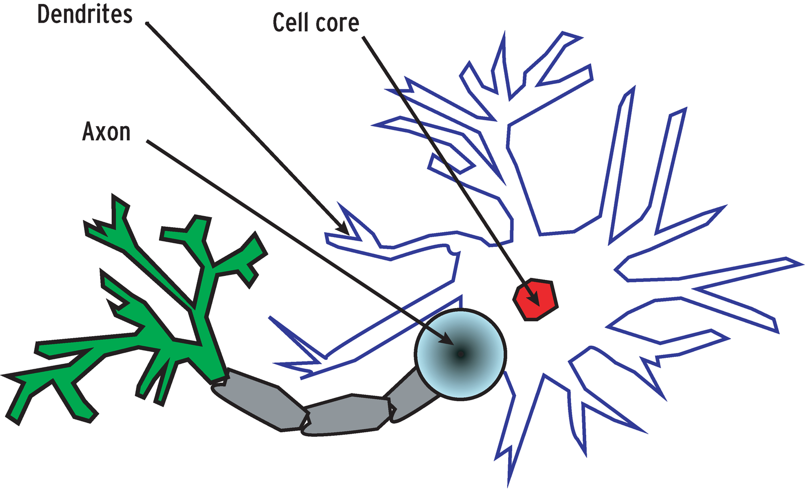
Figure 1 shows a nerve cell, the natural role model for neurons in ANNs. The nerve cell comprises a cell core and dendrites that branch out from it. Dendrites transport electrical impulses to the core of the cell. If the sum total of these impulses exceeds a predefined threshold value (action potential), the neuron becomes active, sending impulses to the cells it is linked with.
An artificial neuron simulates the properties of its natural counterpart: It adds the potentials of its dendrites, applies a fixed activation function, and passes the results to all the cells to which it is linked (Figure 2). Links to other neurons are weighted to attenuate or amplify the signal along its path.
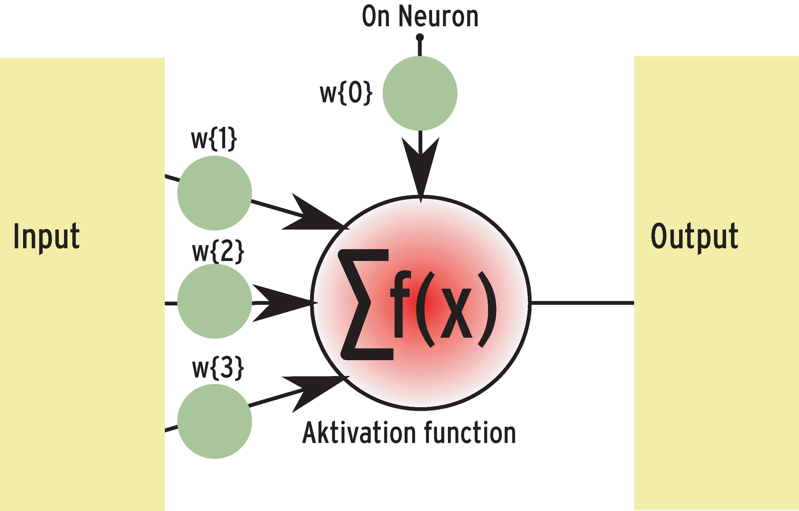
The activation function defines the threshold at which the neuron will activate. Below this value, the neuron will not send signals. This function is often a simple threshold function that returns a 1 if the sum of all outputs is above a specific value. It is common to represent the activation function in a separate neuron known as the on neuron. You can thus weight the on neuron like the links to other neurons.
The training process adapts the neural network for a specific situation; however, at the structural level, the developer must also choose a topology for the neural network that reflects the use for which it is intended. Different types of links between neurons lead to networks with different characteristics [2].
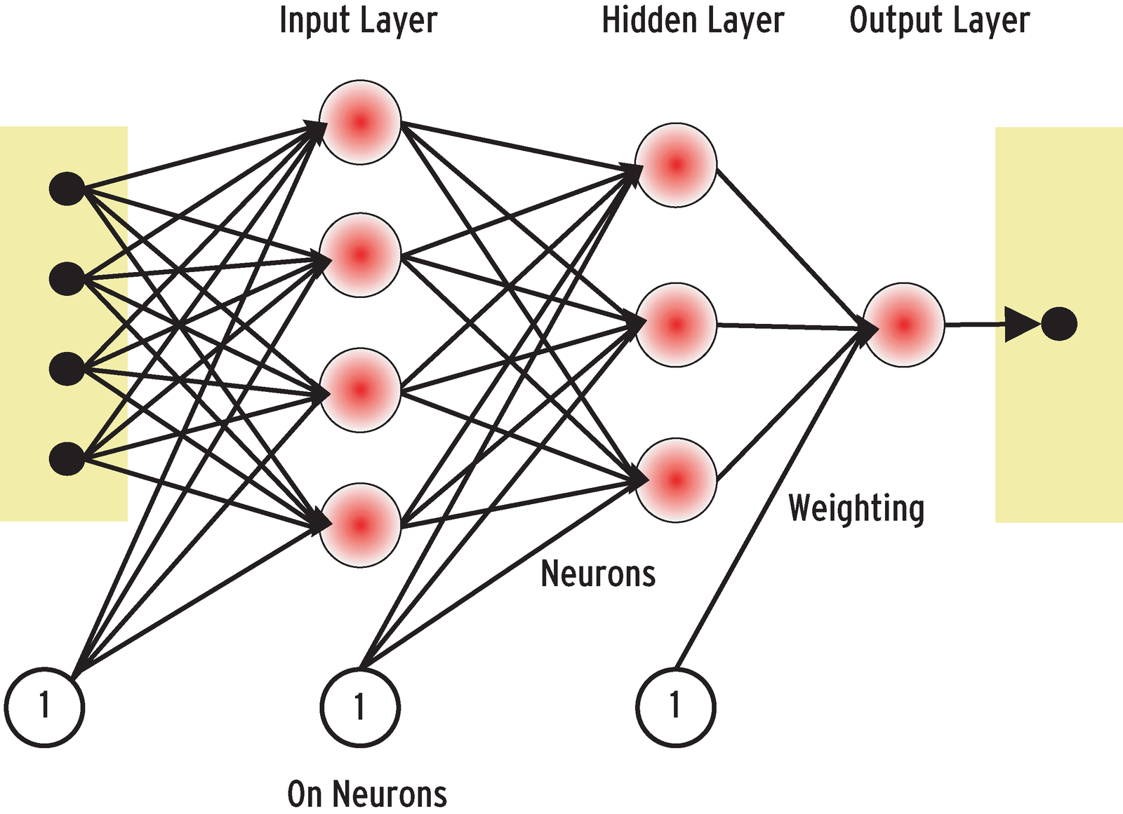
One of the simplest network topologies, and one that is well explored by scientific research, is the feed forward MultiLayer Perceptron (MLP) model [3]. This model divides the network into separate layers. This network has no feedback; in other words, actuation potential simply propagates from left to right (see Figure 3).
A neural network's abilities, such as the ability to recognize patterns or predict values, is a product of the network's internal structure.
The following operations change the characteristics of an ANN:
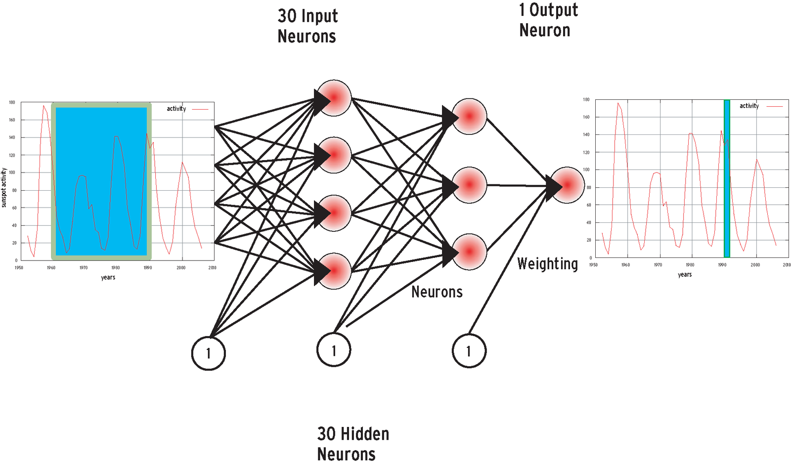
Training provides the right weighting to solve a specific problem. In the case of character recognition, the input would be a bitmap or a section of text and the matching character codes. In the case of stock market behavior or sunspot activity, historic data is used to train the neural network (Figure 6). A learning function compares the example input with the target values and modifies the neuron link, weighting until the reaction of the network matches the target.
I'll use a simple example to describe what happens in a neural network's learning phase. Imagine you want a network with four neurons to predict the mean value of two numbers (see Figure 4). On the left side of the figure, the numbers 0.1 and 0.3 are input at the input neurons. The neural links have random weighting values at first. The activation function, which defines the way a neuron reacts to input, is f(x)=x. More powerful ANNs need more complex functions, of course, but this simple example is adequate to explain the underlying principle.
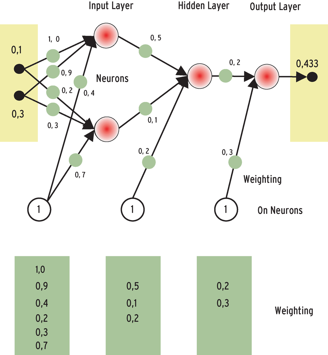
If the input neurons have the values 0.1 and 0.3, weighting the connections for the potentials gives the following values: (0.1*1.0 + 0.3*0.9 + 1.0*0.4) = 0.77 for the first neuron N(1.1), and (0.1*0.2 + 0.3*0.3 + 1.0*0.7) = 0.81, for the second neuron N(1.2). The neuron between the input and output layers has a value of (0.77*0.5 + 0.81*0.1 + 1.0*0.2) = 0.666. The output neuron returns a value of: 0.666*0.2 + 1.0*0.3) = 0.433, although the correct average of the numbers 0.1 and 0.3 is 0.2.
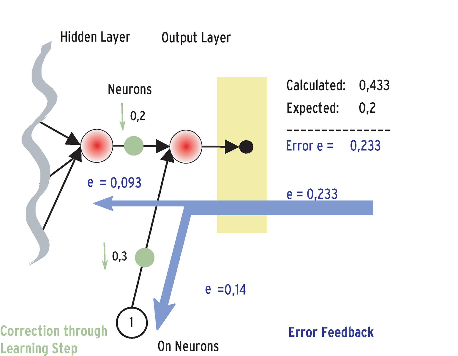
In other words, the network did not come very close to the correct value in this first pass. To allow the ANN to get its math right, I need to modify the weighting for the neural links. The error contribution lets me discover which weighting between which neurons I need to correct. The error contribution is the square of the expected output value, minus the square of the values returned at the output neurons. The resulting value is known as the mean squared error (MSE or MQLE).
Action potentials typically move forward through the network from the input toward the output (feed forward). A teaching method known as back propagation reverses the direction: It feeds the error value returned at the output backward through the network toward the input on the basis of the weighting of the individual connections. The distribution of error values over the nodes of the mesh network provides the basis for modifying the weighting. (The experts have developed several other teaching methods in addition to back propagation, and some methods promise better results for certain tasks.)
Figure 5 shows how the error contribution propagates backward from the output to the input. The potential of the output neuron is the sum of its two links: the link to the on neuron with a weighing of 0.3, and the connection to the neuron in the underlying layer, which is weighted at 0.2. On this basis, the error contribution (0.433 - 0.2 = 0.233) at the output neuron is distributed over the two links. The path to the on neuron has a share of 0.3/(0.2+0.3) = 60%, and the path to the underlying neuron has a share of 0.2/(0.2+0.3)= 40%. This approach provides the ability to calculate the total error potential for each neural link.
Finally, a fixed learning factor stipulates how an error contribution influences the weighting. A good choice of learning factor is a major prerequisite for effective training. Just like many other network parameters, the factor is often unknown until you start training. Complete training of an ANN will always comprise a large number of back-propagation cycles with pairs of input and output values for the problem you need the network to solve after training.
It is obvious that weighting should never be zero because there would be no way of tracing errors back. Too evenly distributed or too widely differing weighting also has a negative effect on the learning process. For an efficient ANN, it is preferable for signals to propagate throughout the whole network except for specific areas of the network to handle specific patterns.
In practical applications, the simple activation function f(x)=x will be replaced by a hyperbolic tangent or a sigmoidal function. This improves the performance of the neural network, as these functions can map an input range to infinity with manageable values. Back propagation also assumes that the activation function can be reversed. The advantage of this extra effort is that three-layer perceptrons are capable of learning arbitrary, mathematic functions, assuming they use suitable non-linear activation functions.
The Fast Artificial Neural Network Library (FANN) is a free, open source library that provides a C interface for implementing multilayer neural networks. The library was developed in 2003 by Steffen Nissen at the University of Copenhagen as part of his scientific research, and it is still under active development. Libfann is easy to use and well documented, and it will run on any popular platform. The project page also has a couple of practical examples that make it easier to get started. Apart from C, there are bindings for all common programming languages. As of this writing, libfann is one of the fastest implementations for neural network simulation.
Most Linux distributions include libfann version 1.2. aptitude install libfann1-dev will install the library on Debian. The source code, which you can build in the usual way, configure; make; make install, is available from [1].
All neural network applications are different, and it is not possible to explore all the subtleties of this complex field in a single article. The libfann project website includes a reference manual with descriptions and usage notes for the functions in the library. See the Linux Magazine website [4] for an example C program that creates a neural network and then goes on to train it.
If you feel like experimenting, a few of the more important libfann functions are fann_train(), fann_run(), and fann_test(). fann_train() expects a network structure, struct fann * ann;, as its first parameter; you can call ann=fann_create(connection_rate, learning_rate, num_layers,num_input, num_neurons_hidden, num_output); to create the structure. The connection_rate specifies the strength of the links between the neurons. The right value is normally 1.0. The learningrate should be between 0.7 and 0.00001. The num_layers parameter, and the values that follow it, tell libfann the number of layers in the network and the number of neurons in each layer.
Parallels to human thinking are useful in understanding what happens during training and in discovering the source of any problems on neural networks - after all, neural networks do emulate the structure of the human brain. If the training session feeds the historic data in chronological order, the network might develop tunnel vision. In other words, the ANN would simply encode the structure of the first or possibly a couple examples in its neurons. This would affect the ANN's ability to handle new data. A random order avoids premature generalization and thus avoids the need to retrain the neural network after an invalid structure is established in the neural links. The Perl script [5] thus ensures a random data order.
Data that the network has not seen during training helps you judge how well the ANN can handle abstractions at the current state of training. The Perl script [5] splits the data into two subsets. The error occurring here is referred to as the mean squared generalization error, or MQGE. Along with the mean squared learning error (MQLE), it tells whether the neural network is ready to predict the future, or whether more training is needed. Libfann injects the two values via the fanntest(ann, inputarray, expected_outputarray) and fann_get_MSE() functions. Finally, fann_save(ann, filename) stores the network structure and the current weighting for future use.
Whether training is successful or not depends not only on the data and the data order, but also on the suitability of the network structure for the task in hand - starting with the activation function. Libfann uses the Sigmoid function by default, and this is fine for predicting sunspot activity and other phenomena that fall in a positive range. For share price variations and other temporal series containing negative values, you will need fann_set_activation_function_output(ann, FANN_SIGMOID), the hyperbolic tangent function.
The learning factor also has a major influence on success or failure of training in that it specifies what effect learning errors have on the weighting of the links between neurons and on the number of neurons on the network. The number of neurons in the intermediate layer should be kept to a minimum at first. Three or a maximum of 15 neurons will be fine for most applications. Trial and error will also give you a gut feeling for appropriate numbers. For this training session, 500,000 learning steps should be sufficient.
If the number of learning errors does not drop continuously, the network is stuck at a local minimum, and its performance is unlikely to improve no matter how long you continue training. In this case, you will need to restart training with a smaller learning factor and possibly change the structure of the network. Inspecting the fann_save file could reveal why you can't improve the performance of a network simply by training: Individual neurons with excessive weighting often interfere with the learning process.
If the learning error continues to drop, as shown in Figure 7, it is time to take a look at the generalization error: If the curve is smooth, you can't expect too much in the line of predictive ability. The network has learned the training values by heart and will be thrown by unknown input values. To change this, you will need to reduce the number of hidden neurons.
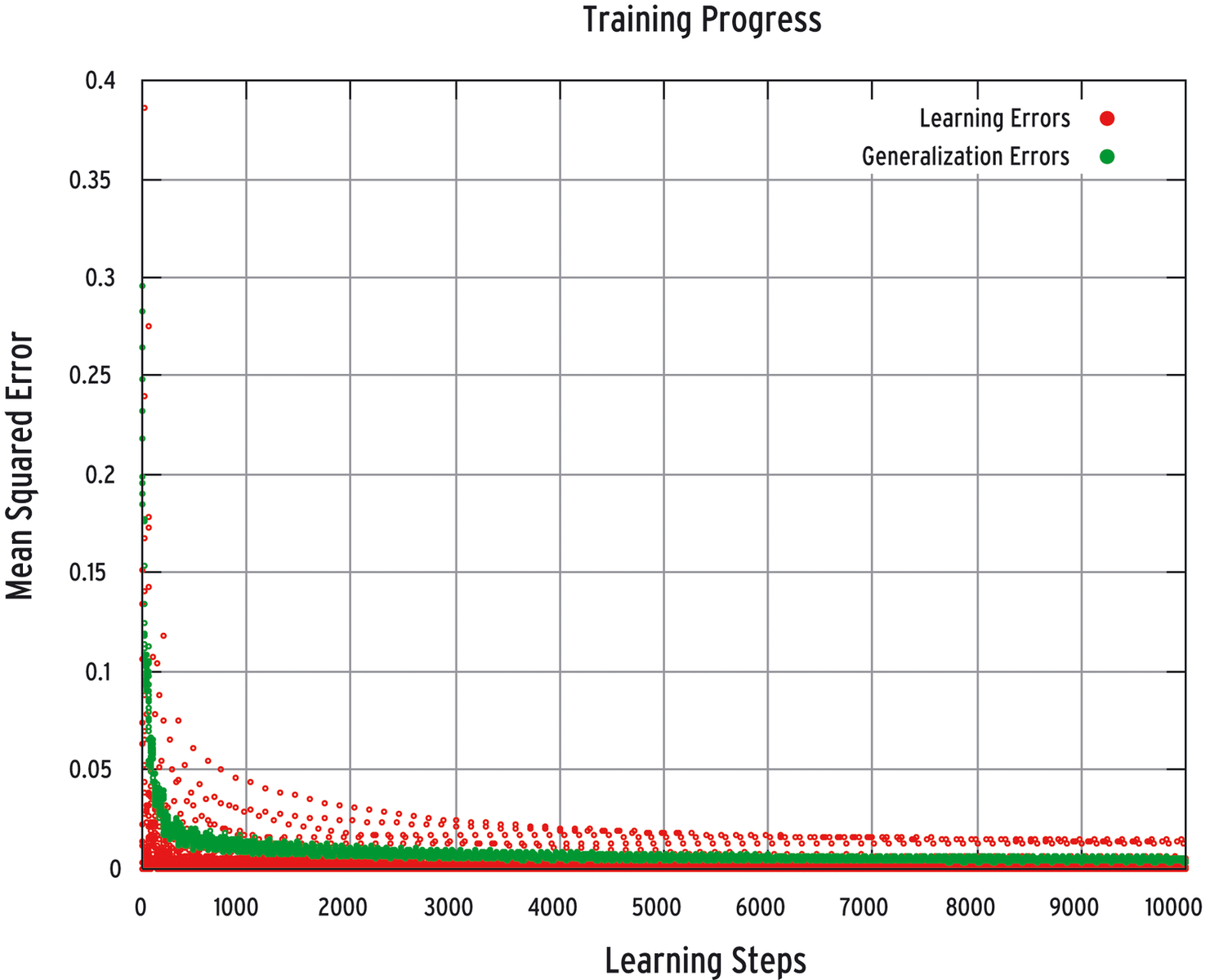
If the generalization error is at a consistently high level, the number of hidden nodes is too low, or the training session was not intensive enough.
Libfann's fann_load loads a network stored previously using fann_save(); fann_run(ann, input) returns the output to the trained network. The Perl script [5] automates a test of the neural brain. In this test, the output from a successfully trained network was pretty close to the predictions.
Libfann makes it easy to set up, train and use ANNs. Users don't need to worry about mathematical details such as inverting the activation function. Choosing parameters such as the learning rate and the number of intermediate neurons does take some experience and patience. The learning error, the generalization error, and an understanding of the saturation of individual neurons will give you some hints as to why training fails for a specific network. Libfann will help you to ascertain these values.
The current version 2.0 of the libfann library extends the functional scope, adding new learning algorithms and neuron types.
| INFO |
|
[1] Libfann: http://fann.sourceforge.net
[2] Neural network types: http://www.neuronalesnetz.de/netztypen.html [3] Multilayer perceptron: http://en.wikipedia.org/wiki/Perceptron [4] C training program: http://www.linux-magazine.com/Magazine/Downloads/83 [5] Perl data preparation script: http://www.linux-magazine.com/Magazine/Downloads/83 [6] Warren Sarle. comp.ai.neural-nets FAQ, http://www.faqs.org/faqs/ai-faq/neural-nets [7] Russell, Stuart and Peter Norvig. Artificial Intelligence: A Modern Approach, 1st ed. Prentice Hall, 1995. |