By Kristian Kißling
If you have ever tried to program a rotating cube in OpenGL, you have probably experienced hours of debugging fun in the process. The lack of libraries and incorrect variable declarations make life hard on amateur programmers.
A graphics programming tool called Processing brings graphic effects back to the everyday user. Processing targets artists who have ideas but no computer science degree. The tool is ideal for users who would like to improve the presentation of their data without having to resort to boring charts and monotonous multi-colored pie diagrams.
The Code Swarm [1] project, for example, uses Processing to visualize the development of various open source projects over the course of time. The fascinating results resemble a beehive, which is sometimes quiet and sometimes populated by large numbers of very active bees.
Processing lets you write a simple program and then just press Play; the code either runs or it doesn't. In the latter case, you are given fairly intelligible feedback to help you troubleshoot. If you want to publish your results on the Internet, you can output a ready-made Java applet at the press of a button, and you can upload it to your web space or web server.
Processing, which first saw the light of day around 2001 at MIT Labs, is often compared with Flash; however, unlike Flash, it is an open source project. Instead of Flash plugins, the viewer simply needs a Java plugin for the browser, an extension that is typically installed in next to no time.
To enjoy the 3D capabilities of the Processing environment, you need either a graphics card with 3D acceleration and driver support or the software 3D engine that comes with the Java application, P3D. The P3D 3D engine needs slightly more in the way of resources than OpenGL, but it is a big help if you do not have a working 3D driver for your graphics card on Linux.
Processing is available for download from the project website [2]. First, unpack the TGZ archive in a folder below your home directory, then pop up a console, change to the directory created in the first step, and enter ./processing to launch the application.
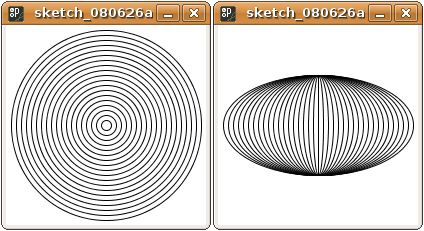
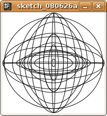
After launching the program, you will see an empty field in which you can start typing code (Figure 1). Why not try it out right way? Just type the program shown in Listing 1 in the window, and then press the icon with the triangle at the top left. Now you should see the object shown in Figure 2 (left).
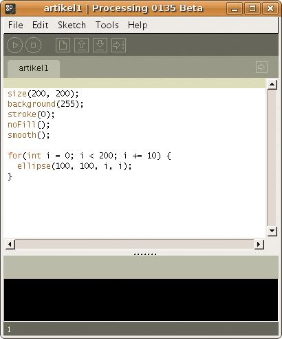
| Listing 1: Drawing a Simple Figure |
01 size(200, 200);
02 background(255);
03 stroke(0);
04 noFill();
05 smooth();
06 for(int i = 0; i < 200; i += 10) {
07   ellipse(100, 100, i, i);
08 }
|
When you run the code in Listing 1, you should see a small window depicting a series of concentric circles. Click Help | Reference in the Processing GUI for a command reference that gives you a short and terse explanation of the individual functions.
If you prefer a more detailed description, select File | Examples to discover one of the many sample programs included with the Processing files. The code is annotated in all cases.
Also, you can find some books on Processing. The tome by Ira Greenberg [3] that I recommend targets artists and non-programmers.
The first two lines of the sample program in Listing 1 open a 200x200-pixel workspace with a white background (background(255)). If you just enter one value, you are selecting one of 255 possible grayscales from 0 (black) to 255 (white). If you enter three comma-separated values, you are specifying the sRGB color space. A background(255, 0, 0) entry would give you a pure red background, for example. To add a black brush stroke, follow the same approach (stroke(0)).
The noFill() function tells Processing not to fill the figures - otherwise the largest circle would cover all the others. An anti-aliasing effect gives smoother edges and is enabled by the aptly named smooth() keyword, which acts on all the following figures. Next, a for() loop executes a specific function until a stop condition occurs (in this case, when i reaches a value of 200).
The loop starts by setting the integer counter to zero (int i =0) and then incrementing in steps of 10 (i+=10). The loop continues while the counter is less than 200 (i < 200). As soon as it reaches the target value, the loop terminates. Each round executes the ellipse() function in line 7. The function draws a circle with the specifications given in the parentheses. The values 100, 100 position the center of the circle at the center of the 200x200-pixel workspace. The two i variables define the vertical and horizontal diameters of the circle. Because i increments in steps of 10, Processing starts by drawing a circle with a diameter of 10, then 20 pixels, and so on.
Small changes can have drastic effects in programming. For instance, if you change the second i in the brackets following ellipse and replace it with 100, as in
ellipse(100, 100, i, 100)
you change the circle to an ellipse (Figure 2, right). While the horizontal diameter continues to grow, thanks to the remaining i, the vertical diameter remains constant at 100 pixels.
The next step adds a random element. Replace the for() loop in Listing 1 with the loop in Listing 2.
| Listing 2: Changing a Parameter |
01 for(int i = 0; i < 200; i += 10) {
02   float r = random(200);
03   ellipse( 100, 100, r, 100);
04 }
|
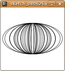
The new loop introduces a new element with the random variable r. In each round, the line float r = random(200); creates a floating point number (float) between 0 and 200 and stores it in variable r. This continually changing number explains the irregular horizontal distances in Figure 3. Adding a second random number (Listing 3) and leaving the vertical diameter to chance (Figure 4) adds more randomness. The figure looks more spatial, but it is by no means three dimensional.
| Listing 3: Adding Randomness |
01 for(int i = 0; i < 200; i += 10) {
02   float r = random(200);
03   float s = random(200);
04   ellipse( 100, 100, r, s);
05 }
|
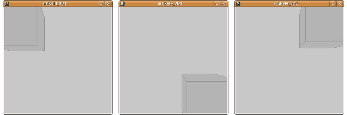
It is quite easy to enter the third dimension with Processing. To demonstrate this, Listing 4 draws a simple cube. The great thing about it is that it reacts to mouse movements - you can push or drag it through the defined workspace (Figure 5). Unfortunately the screenshot tool on Gnome doesn't show you where the mouse is, but you can take my word for it that the mouse was at the center of the cube in all three figures.
| Listing 4: A Simple Cube |
01 void setup() {
02   size(400, 400, P3D);
03   frameRate(30);
04 }
05
06 void draw() {
07   background(200);
08   pushMatrix();
09   translate(mouseX,mouseY,10);
10   color c1 = color(180);
11   fill(c1);
12   stroke(128);
13   box(150);
14   popMatrix();
15 }
|
The code comprises two basic functions: setup() and draw(), which contain other functions. The setup function defines the basic parameters for the program, and the draw function draws a specific object and executes the commands inside the curly brackets before restarting.
The first function in line 2 initializes the workspace; the extent is followed by an ominous looking P3D keyword, which initializes Processing's internal, software-based 3D engine. The engine calculates 3D graphics and sends them to the graphics card, which renders them on screen. To use OpenGL to render the graphic with the use of the faster hardware-based 3D graphics card support, just add the following line at the start of the code:
import processing. opengl.*;
Then replace P3D with OPENGL in Listing 4. On faster machines you will not notice any difference for simple figures.
To see improved performance with more complex figures, you will need a graphics card with 3D acceleration; in other words, you have to install the Nvidia, ATI, or Intel drivers.
Line 3 specifies the frame rate. A value of 30 should be fine, and you will not notice any jerky movements.
The next step relates to the properties of the cube. The example here uses light gray as the background color (background(200)).
The functions pushMatrix() and popMatrix() in lines 8 and 14 draw a framework around the figure. Whereas pushMatrix() creates a new coordinate system and loads it onto the Matrix Stack [4] (see the box titled "What is the Matrix?"), popMatrix() restores the matrix used previously.
Although the program will work without these two functions, they do make sense, as the next example shows.
Inside the matrix, the first function is translate(). It reads the three parameters and positions the cube on the intersection of the x-, y-, and z-axes - that is, in virtual space.
The function assumes a value of 0, 0 for the top left of the workspace and sets the center of the figure to these coordinates.
Any further translate functions that follow inside the draw function will use the previous translation coordinates as their reference point. This means that you can move the cube easily with the mouse because mouseX, mouseY will always relate to the mouse pointer's previous x/y coordinates.
The next trick is to define a color in the variable c1 - light gray in this case, although you can use sRGB values here, too. The script fills the cube with this color in line 11 and colors the edges dark gray by calling stroke().
The cube isn't actually assembled until line 13; the edge length is set to 150 pixels. To draw a cuboid, you need to enter three values for the length, width, and height.
| What is the Matrix? |
|
The following example will give you a rough idea of the Matrix Stack. If you create a series of three sequences, each comprising multiple movements, each sequence starts with the pushMatrix() function, which creates a new coordinate system. To return to the previous sequence, with the previously used coordinates, you just do a popMatrix(). The whole thing works like a kind of return marker, but you can't jump forward. |
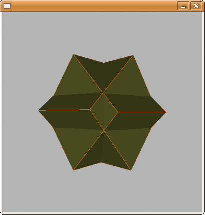
Finally, Listing 5 presents a more complex script. It displays two counter-rotating green cubes (see Figure 6).
| Listing 5: Counter-Rotating Cubes |
01 import processing.opengl.*;
02
03 float ydirection1 = 1;
04 float xdirection1 = 1;
05
06 float ydirection2 = -1;
07 float xdirection2 = -1;
08
09 void setup() {
10   size(400, 400, OPENGL);
11   frameRate(30);
12 }
13
14 void draw() {
15   background(0);
16   directionalLight(255,255,128, 0,0,-1);
17
18 /* Cube 1 */
19   pushMatrix();
20
21   translate(200,200,100);
22   color c1 = color(102, 102, 0);
23   fill(c1);
24   stroke(204,102,0);
25
26   rotateY(radians(ydirection1));
27   rotateX(radians(xdirection1));
28
29   box(100);
30   popMatrix();
31
32 /* Cube 2 */
33   pushMatrix();
34
35   translate(200,200,100);
36   color c2 = color(102, 102, 0);
37   fill(c2);
38   stroke(204,102,0);
39
40   rotateY(radians(ydirection2));
41   rotateX(radians(xdirection2));
42
43   box(100);
44   popMatrix();
45
46 /* cube 1 clockwise */
47   ydirection1 = ydirection1 + 1;
48   xdirection1 = xdirection1 + 1;
49
50 /* cube 2 counterclockwise */
51   ydirection2 = ydirection2 - 1;
52   xdirection2 = xdirection2 - 1;
53
54 }
|
Short comments make the code more intelligible, but the most important features are the use of pushMatrix() and popMatrix() and the commands for rotating the figures.
In lines 3 to 7, I start by initializing two variables for each cube - an xdirection and a ydirection - with values of 1 and -1, respectively. The setup function is already familiar, but the draw function changes.
The script calls directionalLight() to shed some light on the cube. The function has six parameters, the first three of which are for an sRGB or HSV value, and the last three of which are positions on the x-, y-, and z-axes of a spatial coordinate system. The first three values specify the color of the light, and the last three define the direction from which the light comes.
The script defines the size, color, and rotation of the two cubes between the pushMatrix() and popMatrix() functions. The functions are the same for both cubes apart from one detail: The rotateX() and rotateY functions use opposite directions of rotation.
Lines 40 and 41 rotate cube 2 one degree counterclockwise on the x- and y-axes. Both variables start with a value of -1. Cube 1 rotates in the opposite direction. Because they are centered on the same position, they counter-rotate. After this minimal rotation, new values are assigned to the variables in lines 46 to 52.
The torque is incremented for cube 1 and decremented for cube 2. Processing executes the draw function again, and both cubes counter-rotate another degree. Because the draw function uses a frame rate of 30 frames per second, the cubes rotate smoothly.
One other interesting aspect might interest you: If you remove the pushMatrix() and popMatrix() functions in the sample code, the second cube suddenly orbits the first like a planet. Each cube would need a separate coordinate system - unless you want to design a virtual planetarium.
By default, Processing stores your efforts in a folder titled sketchbook below your home directory. If you save your creation as experiment_0815, you would find it later in ~/sketchbook/experiment_0815/.
To show off your programming skills to friends, colleagues, and acquaintances, you might want to publish your figures on the web. Selecting File | Export lets you do so. Processing will then create an applet subfolder below the above-mentioned directory and drop the required files into it. If you open the index.html file in your browser, you should see the figure.
To publish the figure on your homepage, just use an FTP client to push the applet folder onto the server with your website and add a link to index.html to your homepage.
If you want to access the file directly, just go to http://www.mydomain.com/applet/index.html.
| INFO |
|
[1] The Code Swarm project uses Processing: http://code.google.com/p/codeswarm/
[2] Download page for Processing: http://processing.org/download/index.html [3] Greenberg, Ira A. Processing: Creative Coding and Computational Art. Computer Bookshops, New York, 2007. [4] pushMatrix() and popMatrix() explained: http://processing.org/discourse/yabb_beta/YaBB.cgi?board=Syntax;action=display;num=1177279317 |
| THE AUTHOR |
|
Kristian officially studied german philology, history and social science in Berlin but wasted a lot of his time with computers. He got hooked on Linux in the 90ies and works now as editor for LinuxUser. |