By Michael Schilli
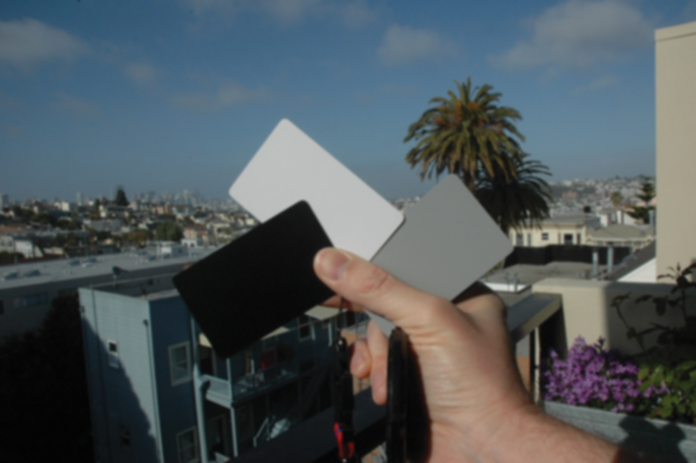
Last month, I wrote about using reference cards to correct the white balance in digital photos by taking a test snapshot (see Figure 1) [2]. The black, white, and gray plastic cards, which are available from any good photography equipment dealer, should not generate any color values in a digital image. This provides three calibration points for low, medium, and high light intensity, which the GIMP photo editing tool can then reference to correct your snapshots.

How can a simple Perl script find out which pixel values the three cards create, even though their position in the image is not known, without using artificial intelligence?
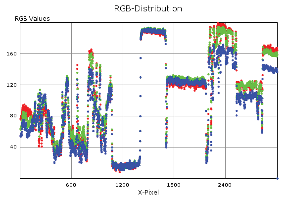
If the photographer manages to spread the cards in the center of the image as shown in Figure 1, the script can follow an imaginary horizontal line and identify the cards on the basis of pixel values along the x axis.
The light intensity measured along this line remains constant for a fairly substantial distance, as long as the line lies within one reference card.
Once the line touches the background, the pixel values will start to fluctuate significantly.
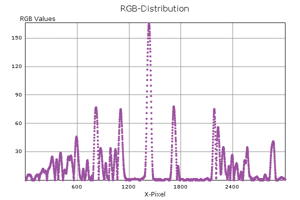
Listing 1, graphdraw, uses the CPAN Imager module to create the graphs shown in Figure 2.
The graphs represent the red, green, and blue components of the color values along the horizontal line drawn in Figure 1 on a coordinate system in which the x axis matches the x coordinates in the image and the y value represents the color component value with a range of 0 through 255.
The CPAN Imager module's read() (line 12) is a multi-talented beast that can identify, read, and convert any popular image format to its own internal Imager format for editing.
| Listing 1: graphdraw |
01 #!/usr/local/bin/perl -w
02 use strict;
03 use Imager;
04 use Imager::Plot;
05 use Log::Log4perl;
06
07 my ($file) = @ARGV;
08 die "No file given"
09   unless defined $file;
10
11 my $img = Imager->new();
12 $img->read( file => $file )
13   or die $img->errstr();
14
15 $img->filter(
16   type   => "gaussian",
17   stddev => 10
18 ) or die $img->errstr;
19
20 my $y = int(
21   $img->getheight() / 2 );
22 my $width = $img->getwidth();
23
24 my $data = {};
25
26 for my $x ( 0 .. $width - 1 )
27 {
28   push @{ $data->{x} }, $x;
29
30   my $color = $img->getpixel(
31     x => $x,
32     y => $y
33   );
34   my @components =
35     $color->rgba();
36   for my $color_name (
37     qw(red green blue))
38   {
39     push @{ $data
40         ->{$color_name} },
41       shift @components;
42   }
43 }
44
45 my $plot = Imager::Plot->new(
46   Width  => 550,
47   Height => 350,
48   GlobalFont =>
49 ,/usr/share/fonts/truetype/msttcorefonts/Verdana.ttf'
50 );
51
52 for my $color_name (
53   qw(red green blue))
54 {
55   $plot->AddDataSet(
56     X => $data->{x},
57     Y =>
58       $data->{$color_name},
59     style => {
60       marker => {
61         size   => 2,
62         symbol => ,circle',
63         color =>
64           Imager::Color->new(
65           $color_name),
66       }
67     }
68   );
69 }
70
71 my $graph = Imager->new(
72   xsize => 600,
73   ysize => 400
74 );
75
76 $graph->box(
77   filled => 1,
78   color  => ,white'
79 );
80
81 # Add text
82 $plot->{,Ylabel'} =
83   ,RGB Values';
84 $plot->{,Xlabel'} =
85   ,X-Pixel';
86 $plot->{,Title'} =
87   ,RGB-Distribution';
88
89 $plot->Render(
90   Image => $graph,
91   Xoff  => 40,
92   Yoff  => 370
93 );
94
95 $graph->write(
96   file => "graph.png" )
97   or die $graph->errstr();
|
If something goes wrong, the Imager methods return false values. For more details about an error, cautious programmers tend to call the errstr() method to return a cleartext description of the issue. The getpixel() method (line 30) examines the RGB values of a pixel in the image at a location defined by its x and y coordinates and returns an Imager::Color object, which contains the pixel's RGB values.
A call to rgba() (line 35) returns these values along with the value for the alpha channel. Here, you are just interested in the first three RGB values.
The script calls shift in line 41 to extract them one by one.
The Imager::Plot module represents boring numbers as graphs in an attractive coordinate system without too much hassle with respect to scaling, axis labeling, or graphical layout, and it returns image files in all popular formats, allowing the user to check them later with an image viewer or web browser. The new() constructor (line 45) accepts the dimensions for the resulting image and the path to an installed True Type font, which it then uses for axis labeling.
The script collects the required coordinates in a hash of hashes, to which $data points. It stores all the x coordinates in $data->{x} and all red values in $data->{red}; the green and blue values are stored in the same manner. The AddDataSet() method (line 55) then adds the data separately for each of the three graphs, each of which are drawn in a different color.
On completion, a new Imager object is created in line 71; later, it will create the resulting graphics file. Before this happens, the box() method colors the image background white, then Render() draws the coordinate system, the labels, and the three graphs in one fell swoop.
Finally, the write() method saves the output file on disk in PNG format.
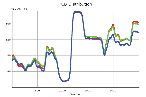
Before a script can reliably identify the three areas at the center of the image, you need to make some preparations. Figure 2 clearly shows how much the graph fluctuates, and this is obviously going to make it difficult to identify the somewhat flatter areas. Thus, the cardfind detection script (Listing 2) needs to run a blur filter that uses the "Gaussian Blur" method with a radius of 10 to defocus the image (lines 15ff.).
In an out-of-focus image (see Figure 3), the color transitions between individual pixels are less abrupt. Instead of jumping directly from a white to black pixel, an out-of-focus image will show a transition with several gray scale values. The graph shown in Figure 4, which represents the pixel values on the same horizontal line, is far smoother as a result of this, and also simplifies the task of identifying the three areas to be identified.
| Listing 2: cardfind |
001 #!/usr/local/bin/perl -w
002 use strict;
003 use Imager;
004 use YAML qw(Dump);
005
006 my ($file) = @ARGV;
007 die "No file given"
008   unless defined $file;
009
010 my $img = Imager->new();
011 $img->read( file => $file )
012   or die "Can't read $file";
013
014 # Blur
015 $img->filter(
016   type   => "gaussian",
017   stddev => 10
018 ) or die $img->errstr;
019
020 my $y = int(
021   $img->getheight() / 2 );
022 my $width = $img->getwidth();
023
024 my @intens_ring = ();
025 my @diff_ring   = ();
026 my $found       = 0;
027 my @ctl_points  = ();
028
029 for my $x ( 0 .. $width - 1 )
030 {
031   my $color = $img->getpixel(
032     x => $x,
033     y => $y
034   );
035   my @components =
036     $color->rgba();
037
038 # Save current intensity
039 # in ring buffer
040   my $intens =
041     @components[ 0, 1, 2 ];
042   push @intens_ring, $intens;
043   shift @intens_ring
044     if @intens_ring > 50;
045
046 # Store slope between
047 # x and x-50
048   push @diff_ring,
049     abs( $intens -
050       $intens_ring[0] );
051   shift @diff_ring
052     if @diff_ring > 50;
053
054   if ($found) {
055
056     # Inside flat region
057     if ( avg( \@diff_ring ) >
058       10 )
059     {
060       $found = 0;
061     }
062   }
063   else {
064
065     # Outside flat region
066     if (  $x > $width / 3
067       and $x < 2 / 3 * $width
068       and avg( \@diff_ring )
069       < 3 )
070     {
071       $found = 1;
072       push @ctl_points,
073         [ @components[ 0, 1,
074         2 ] ];
075     }
076   }
077 }
078
079 my $out = {};
080 my @labels =
081   qw(low medium high);
082
083 # Sort by intensity
084 for my $ctl_point (
085   sort {
086     $a->[0] +
087       $a->[1] +
088       $a->[2] <=> $b->[0] +
089       $b->[1] +
090       $b->[2]
091   } @ctl_points
092   )
093 {
094   my $label = shift @labels;
095   $out->{$label}->{red} =
096     $ctl_point->[0];
097   $out->{$label}->{green} =
098     $ctl_point->[1];
099   $out->{$label}->{blue} =
100     $ctl_point->[2];
101   last unless @labels;
102 }
103
104 print Dump($out);
105
106 #############################
107 sub avg {
108 #############################
109   my ($arr) = @_;
110
111   my $sum = 0;
112   $sum += $_ for @$arr;
113   return $sum / @$arr;
114 }
|
In these card areas, the curve is fairly flat over a length of hundreds of pixels. If you remember your math from school, you might recall that the first derivative of a graph like this at flat spots is constant and about zero, whereas the values will be far higher and fluctuate significantly everywhere else.
Figure 5 shows the first derivative of intensity values, which are calculated by adding the pixel values for the red, green, and blue channels. The recorded values are indicative of the fluctuation of the original graph and drop to zero over quite considerable distances.
The cards, with their homogeneous gray scales, occupy these positions in the original image. Thus, the script just needs to follow this graph, create a ring buffer of about 50 investigated values, and alert when the buffer average drops to a value close to zero. When it does so, it has located a card.
When the buffer values start to fluctuate again, the script has left the card area and returns to the state "search for the next homogeneous location." The script should be able to find all three regions you are looking for and return the RGB values it finds there in YAML format. This lets the picfix script I discussed in last month's Perl column adjust the white balance of other images with the same light conditions.
The photographer still needs to repeat the reference card shot whenever the scene changes. All following photos of the same scene can then be corrected by GIMP and the picfix script.
To make sure this approach works even if the snapshot happens to have a fairly homogeneous background, lines 66 through 68 not only check to see whether the mean value in the buffer is less than 3, but also whether the algorithm is in the middle third of the image, ignoring the left and right thirds.
The script uses normal Perl arrays as ring buffers and uses push() to append new values before checking to see whether the array exceeds the maximum length of the buffer. If this is the case, it deletes the first array element by calling shift(). This shortens the array by one element, and the second element moves up to the first spot.
To calculate the first derivative of the fairly complex pixel function, you can use a simplified numeric approach.
The ring buffer, @intens_ring, stores the intensity values of the last 50 pixels, which were created by adding the red, green, and blue values at the processed x coordinates.
To extract the three values from the four-element list returned by the rgba() method (line 36), the script relies on the array slice technique @components[0,1,2] (line 41). The value of the first derivate - that is, the slope of the graph at this point - is then approximated as the difference between the first and last elements in the ring buffer at constant distance x. Positive or negative slopes are of no interest, so abs() converts them to positive values if needed.
To find out whether the algorithm is currently in one of the flat parts of the graph that are being investigated, or in a more mountainous region, the script sets up a second ring buffer, @diff_ring, which contains the last 50 values determined for the first derivate of the graph (lines 51, 52). The avg() function defined in line 107ff. calculates the mean value of 50 intensity values. If the algorithm is currently in a peaky region, a mean value below a threshold of 3 is all you need to identify a flat part.
Once the script hits a flat area, it takes a mean increase of more than 10 to convince the state machine that it is back in the mountains.
Each time the script identifies a flat area, line 72 stores the RGB values of the first pixel found in this area in the @ctl_points array. Because you are only interested in three flat spots; the last instruction in line 101 scraps any others.
Finally, the Dump() function from the YAML module from CPAN outputs the results (Figure 6) in the form of a YAML file, sample.yml.
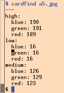
Storing the results and passing them in to last month's picfix script as -c sample.yml lets you correct the color casting in the image with the cards, and any number of images you took with the same lighting - but don't forget to hold the cards in the middle of the photo to make sure that the simple algorithm finds them. To find the cards otherwise, you would need a far more sophisticated algorithm.
On the other hand, Perl, with its treasure of modules on CPAN, gives you ample fodder for your experiments.
| INFO |
|
[1] Listings for this article: http://www.linux-magazine.com/resources/article_code
[2] "Color Play" by Michael Schilli, Linux Magazine, September 2008: http://www.linux-magazine.com/issues/2008/94/color_play |
| THE AUTHOR |
|
Michael Schilli works as a Software Developer at Yahoo!, Sunnyvale, California. He wrote "Perl Power" for Addison-Wesley and can be contacted at mschilli@perlmeister.com. His homepage is at http://perlmeister.com. |