
By Thomas Romeyke
The Maxima [1] Computer Algebra System (CAS) is a free tool for solving and simplifying mathematical equations. Originally created in the 1960s as a commercial program (Macsyma), Maxima is now included by many Linux distributions, although a Windows version is also available.
Maxima's preference for the command line reveals its Unix roots, but if you prefer a GUI, never fear. WxMaxima [2] offers a Maxima GUI interface that provides menus, mouse input, and graphical output.
In the simplest of all cases, you can use Maxima just like a pocket calculator: typing 101*27 at the prompt will give you 2727. Input starts with a prompt of %i (for input), and output with %o (for output).
The output window numbers the lines and gives you the ability to perform further computations on previous results. For instance, to divide the result of this first simple example by 84, just enter %/84; the percent sign represents the last output.
To calculate with older results, type the line number after the percent sign, for example, %o3. The result of this first experiment might surprise you, 2727/84 results in 909/28 - the fraction is mathematically reduced to its simplest form.
To request decimal notation, add numer (for numeric) to the calculation. This option gives you a 16-digit approximation with the last digit rounded. If this is not accurate enough for you, you can specify a degree of floating point precision of 60 with the command fpprec:60, which is available in the menu at the top below Numeric.
Then you must typecast the result as a big float, using bfloat(%) or bfloat(909/28).This approach lets you view as many decimal places as you like, but only makes sense for fractions with very short periods.
If you really want to see the first 3,000 decimal places of pi (Maxima has a %pi constant for this), you would just type fpprec:3000, followed by \%pi,numer.
Of course, the system can resolve fractions. Entering:
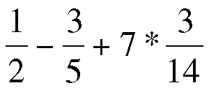
outputs the exact result: 7/5.
Maxima is available from its homepage on Sourceforge [1] for Linux and other operating systems. The current version is 5.14.0. Most Linux distributions include Maxima and the wxMaxima GUI by default. On Ubuntu 8.04, for example, users can just apt-get install maxima wxmaxima gnuplot to install the full set of packages. Unfortunately, the Ubuntu repository only offers the second-to-last version - although this should be fine for getting started. If necessary, you can download the source code or the latest RPM package from the Maxima page [2].
Another typical Maxima task is precise calculations with very large numbers. Pocket calculators and spreadsheets automatically switch to an exponential notation as of a certain size of number (for example, 231).
In contrast to this, wxMaxima gives users the ability to calculate with numbers of any size; the limit is basically defined by the amount of RAM you have available.
For example, the program has no trouble writing out the number 2170:
1496577676626844588240573268701473812127674924007424
wxMaxima just outputs the first and last digits in even larger numbers and lets you know the total number of digits. For example, 13220 results in a number with about 250 digits, of which just the first and last 30 are output.
If you want to see all the digits, you can do so by issuing the set_display(ascii) command. The factorial of 1,500 (1500!) will fill the screen with a number comprising over 4000 digits. To restore the more convenient reduced notation, just tell Maxima to set_display(xml).
The program implements not only the factorial function, but also a number of prime number functions that allow for interesting experiments, especially in combination with calculations involving large numbers. For example, the primep() function checks whether a number is a prime number. primep(788367353713) returns true (the number is a prime number), whereas a test of 788367353643 returns false.
Factoring tells you which prime factors the second figure comprises: factor(788367353643) returns the factors 3 * 3 * 733 * 119503919. A number built out of many prime factors will give you a far more impressive list: try factor(5000!).
Searching for a large prime number (which is sometimes necessary with cryptographic applications) is fairly simple. The instruction p1:next_prime(377220) finds the first prime number that follows 377220 and stores it in a variable dubbed p1 - this is a figure with about 500 digits.
Calling the function p2:next_prime(%) finds the next prime number and stores it as p2. Depending on your computer, this could take a couple of seconds.
The product of the two prime numbers (p1*p2) is a useful basis for part of an RSA key. However, using consecutive prime numbers is not recommended in production environments.
The following is an example of a composite number:
345862011780410397876013873188202447214134147993527728038112440197322495509204470242935323783165385289930823657232278711064866624396026528162520366869362889027847958124572048492902238930631589988184826133619274368192339977782807717735312582897230196328769838321209122609377462417318508826015697895512065549020013940594309185368543866142627334637083672548438918468553728549604911185025083035795738981546908678540702875792312840910506614178563476224312376011581158579070227159596612897837865541697908514794385246878768150137301974631020508238553705918725815721502791333002836671068519210347427534113281007898764644175589677906569910366868727657616275090844456345270852746790478521245034979650230712487412014882245913487037099190364226621719562272089742807613919578158325332361890921677816966011968781104142713267093080704641916493691780983794152328256135894898253264957641101560408631873470108837849577534668782072859228734103104199834644775463040487237495558910707470179588781884923881018390446977360885215482029883283976880008163640733890944133463087709320026714183311160400564555642278016518244662185883042717413
Again, this number is the product of two large prime numbers. If you don't need your computer for a while, you can ask it to discover the prime factors.
Automatic manipulation of algebraic expressions is a fascinating example of a field in which Maxima draws on a collection of mathematical knowledge implemented over a period of decades. To avoid tripping over what - at first glance - appears to be a quirky approach to sorting variables in the output, you might want to take control of how the variables are output. The following example uses the variables a, b, c, d, x, y, and z. The command ordergre-at(a,b,c,d,x,y,z) forces this order in the output. When you type
![]()
Maxima displays the expression in a visually attractive way:
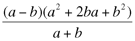
Like other CAS systems, wxMaxima supports methods that apply mathematical laws to simplify algebraic expressions, typically by means of sophisticated rephrasing and reducing. The example here uses the ratsimp(%) command. wxMaxima identifies the binomial formula, converts appropriately, and reduces the results to a very simple expression a2 * b2.
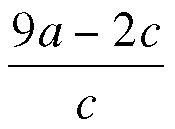
wxMaxima shows ((9*a-c)/c)+((7*a-2*b)/(2*b-7*a)) as:
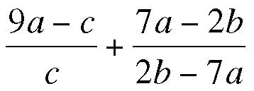
Calling the Ratsimp simplification method creates the following equivalent expression:
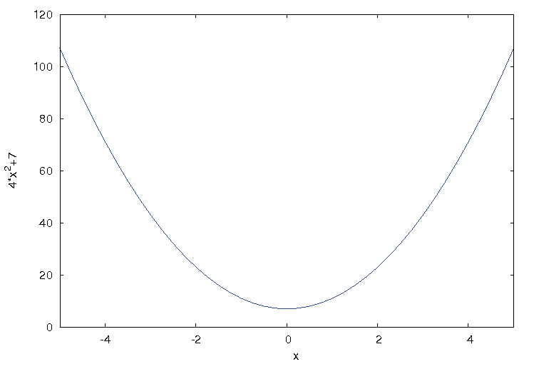
Graphical output of function curves (plotting) is another useful feature. wxMaxima relies on the popular Gnuplot package for plotting. To access the Plot menu, you have two options. The top menu bar includes a number of useful subitems below Plot, but you can just as easily press the 2D Plot button in the lower part of the screen. The top line of the dialog expects the function to plot: 4*x2+7. You can leave the other settings as is for the time being. Clicking OK displays the graph shown in Figure 1.
In many cases, a user might want to simply change a couple of graphics parameters. A simple trick to avoid the need to enter the same values time and time again in the dialog is clicking the line that produced the last plot command to tell the plot function to apply the same values the next time you call it. Then you can change the values individually.
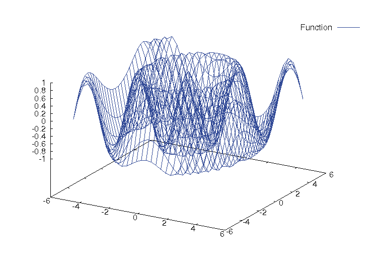
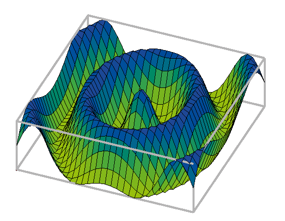
Some functions with two independent variables result in interesting graphs. The 3D Plot menu item lets you plot three-dimensional graphs. The example in Figure 2 shows the output of the function cos(sqrt(5*x2 + 3*y2)). In this case, it makes sense to choose the Openmath output format. This not only opens a new window for the graph but lets you use the mouse to rotate, zoom, and scale the output (Figure 3).
Maxima is not just a tool for mathematical experiments; it can help you solve genuine problems, as the next simple example shows.
For an example of Maxima in the real world, consider a chemical manufacturer who produces two liquid products (P1 and P2), which are sold with different profit margins (PM-P1 = EUR 95 and PM-P2 = EUR 75). Both products are made up of four component products (C1 to C4) - these component products might represent color components.
A precisely defined mixing ratio is required for both of the products: the vector P1(3; 1; 3; 11) specifies that to produce one unit (UN) of P1, exactly three units of V1 are required, whereas just one UN of V2 is required. The vector for the other product is P2(1; 5; 2; 2). The example also assumes that resources of the component products are limited. The plan thus needs to take the existing stocks S of the component products into consideration: S(260; 575; 320; 920).
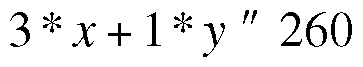
On the basis of this data, it is possible to generate a mathematical model, which Maxima can solve by linear optimization. The first thing is to define the target function. It is safe to assume that the planner will want to maximize the profit margins generated by P1 and P2:
![]()
The values x and y represent the number of units to produce. The remaining details in this example are defined as auxiliary conditions that ensure the solution is physically possible. In the case of component product C1, each unit of P1 will consume exactly three units of C1. On the basis of the same system, each unit of P2 consumes one unit of C1, and so on. Because only 260 units of C1 exist, the first auxiliary condition is:
On the basis of the same reasoning, you can apply three further auxiliary conditions. First, add two more to prevent x and y from assuming negative values, because a negative quantity can't exist in real conditions in many situations:
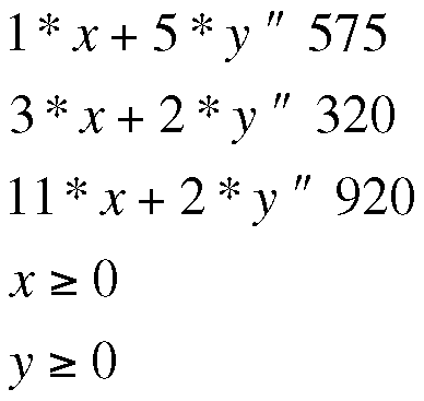
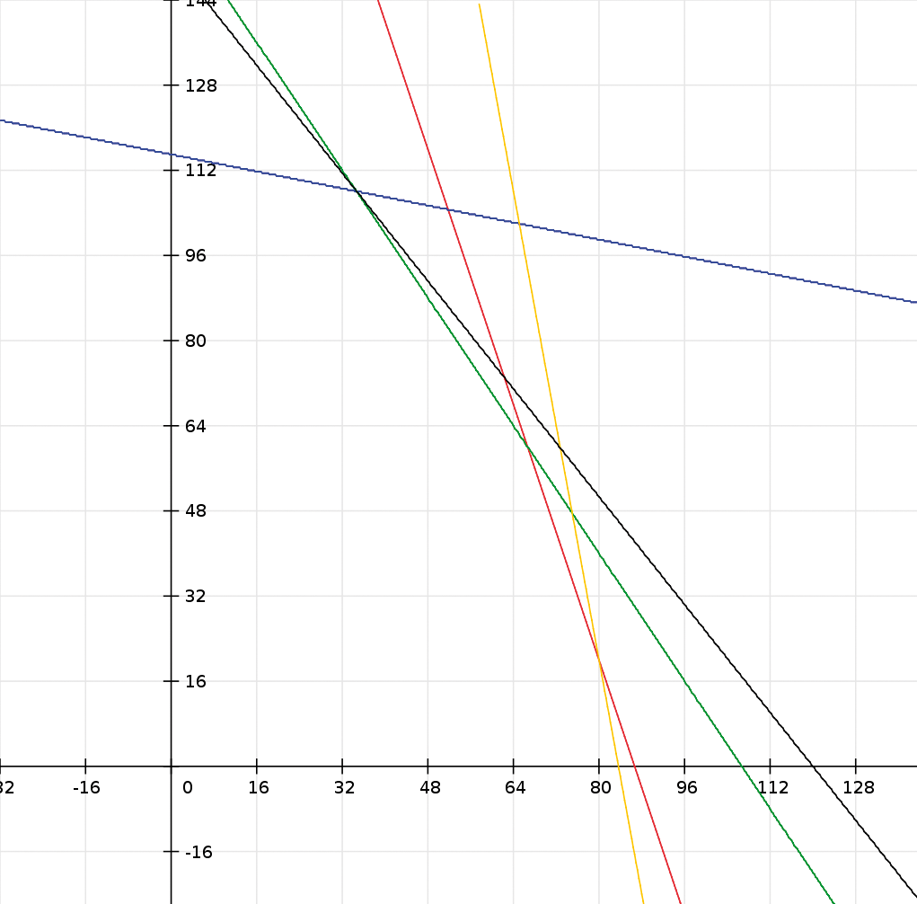
Figure 4 shows the coherencies: the polygon between the x and y axes and the colored straight lines containing all possible combinations of solution for optimizing production. The most favorable combination will be at the top, far right. The black target function is drawn to intersect some of the auxiliary conditions at the optimum point, and you want Maxima to calculate this point.
To simplify changes, all the details are stored as variables:
Tf: 95*x + 75*y
Con1: 3*x + y <= 260
Con2: 1*x + 5*y <= 575
Con3: 3*x + 2*y <= 320
Con4: 11*x + 2*y <= 920
Con5: x >= 0
Con6: y >= 0
As the first step toward an optimized solution, you first need to load the Simplex module using the Maxima load(simplex) command. Then you can call the function maximize_sx(Tf; [Con1;Con2;Con3;Con4;Con5;Con6]) and pass in the target function and the auxiliary conditions to it. The results show that producing 34.6 units of P1 and 108 units of P2 would result in the perfect profit margin of EUR 11,394. The Maxima manual still refers to this function as maximize_lp(); however, maximize_sx() replaced it years ago. In a similar way, the minimize_sx() function handles minimization. The Simplex method implemented by Maxima is extremely powerful.
The number of variables and auxiliary conditions can be very large, again depending on the amount of RAM you have available. This puts relatively small computers with the free Maxima program in a position to solve optimization tasks that would have kept a mainframe busy for hours just 20 years ago.
This short excursion into the world of Maxima can't replace a thorough review of the Maxima manual - the PDF document has no fewer than 800 pages. Some commercial competitors might have more modern input and output methods, but from a mathematical point of view, Maxima can easily keep pace with its more expensive siblings.
Easy availability is another argument in favor of using Maxima at home, school, and college. Anybody can install the software in next to no time - and there's no need to purchase an expensive license.
| INFO |
|
[1] Maxima homepage: http://maxima.sourceforge.net
[2] wxMaxima homepage: http://wxmaxima.sourceforge.net |