
Nicolas Dichtel and Thierry Herbelot pointed out that the directories in the /proc filesystem used a linked list to identify their files. But, this would be slow when /proc directories started having lots of files, which, for example, might happen when the system needed lots of network sockets.
Nicolas and Thierry posted a patch to change the /proc implementation to use multiple linked lists instead of just one. Each subdirectory would have its own linked list, keyed to a hash of the directory's name. According to their benchmarks, the patch shaved 1/5 of the time needed to churn through all the entries of a given subdirectory.
Stephen Hemminger liked the speedup, but suggested that there already were implementations, like the hlist macro, that might simplify their hash table code.
Eric W. Biederman also liked the speedup and kicked himself for overlooking the /proc issue when doing other scalability work. But, he felt that the whole linked list concept was not the right approach. Especially, he felt that /proc/net/dev/snmp6 was the real target of Nicolas and Thierry's patch, and if no one actually needed the files in that directory (except people requiring extreme backward compatibility), it would be even more efficient to do away with them completely.
This, however, already had come up in an earlier thread, when David S. Miller had said that “It potentially breaks tools, it's a non-starter, sorry.” So, reworking the user interface would not be allowed, which left the linked list speedup that Nicolas and Thierry proposed. But, Nicolas said he'd look into an rbtree implementation instead of a plain linked list, because rbtrees would potentially scale better.
Minchan Kim noticed that putting memory pressure on qemu-kvm under Linux 3.14 would cause a kernel stack overflow and crash the system. He dug into the code and tried to reduce his own stack usage, but he wasn't able to cut back enough to prevent the crash. And in any case, he said, trying to reduce everyone's stack usage was not very scalable. He proposed expanding the kernel stack from 8K to 16K, although he acknowledged that there possibly were good reasons not to do this that he wasn't aware of.
Dave Chinner remarked that “8k stacks were never large enough to fit the Linux IO architecture on x86-64, but nobody outside filesystem and IO developers has been willing to accept that argument as valid, despite regular stack overruns and filesystems having to add workaround after workaround to prevent stack overruns.”
He added, “We're basically at the point where we have to push every XFS operation that requires block allocation off to another thread to get enough stack space for normal operation”, and said “XFS has always been the stack usage canary and this issue is basically a repeat of the 4k stack on i386 kernel debacle.”
Borislav Petkov pointed out that if they increased the kernel stack from 8K to 16K, there undoubtedly would come a time when 16K wouldn't be enough either. He wondered if there ever would be a limit, or if the kernel stack ultimately would grow to one megabyte and beyond.
Steven Rostedt said, “If [Minchan's patch] goes in, it should be a config option, or perhaps selected by those filesystems that need it. I hate to have 16K stacks on a box that doesn't have that much memory, but also just uses ext2.”
Meanwhile, H. Peter Anvin said, “8K additional per thread is a huge hit. XFS has indeed always been a canary, or trouble spot, I suspect because it originally came from another kernel where this was not an optimization target.”
At around this point, Linus Torvalds remarked that something like Minchan's fix probably would be necessary at some point, although the development cycle was already at -rc7, making it too late for that particular kernel version. Linus also pointed out that there was plenty of room to reduce stack usage in the stack trace Minchan had posted in his original e-mail. Linus remarked, “From a quick glance at the frame usage, some of it seems to be gcc being rather bad at stack allocation, but lots of it is just nasty spilling around the disgusting call-sites with tons or arguments. A lot of the stack slots are marked as '%sfp' (which is gcc-ese for 'spill frame pointer', afaik).”
There was a technical discussion about various ways to reduce stack usage in general (and some further consideration of ways in which GCC might be somewhat to blame), but with Linus willing to accept a patch to implement a larger stack, it seems like something along the lines of Minchan's patch will soon be part of the kernel. At one point, Linus summed up his position on the issue, saying, “Minchan's call trace and this thread has actually convinced me that yes, we really do need to make x86-64 have a 16kB stack. [...] The 8kB stack has been somewhat restrictive and painful for a while, and I'm ok with admitting that it is just getting too damn painful.”
I love my latest Android device (see this issue's Open-Source Classroom column for details), but for some reason, it won't automatically connect to my Bluetooth headset. When I turn on my headset, I want it to connect to my Android device so I can start using it right away. In order to make it connect, I have to go into the settings app, then Bluetooth, and then tap the device to connect. Thankfully, there's an application that makes life a lot easier.
Bluetooth Auto Connect is a program that runs in the background. It doesn't constantly poll for newly turned on Bluetooth devices, because that would waste battery power. It has several other ways to initiate the connection though. My favorite is the “connect when powered on” option. Because I always have to turn the phone on in order to start my audiobook (or music), it's not an inconvenience to turn the screen on in order to connect Bluetooth. As soon as the power button is pressed, it connects to my headset, and by the time I open the media player application, it's ready to rock!
Sometimes it's the simplest applications that are the most useful. Bluetooth Auto Connect is one of those. Check it out in the Google Play Store today: https://play.google.com/store/apps/details?id=org.myklos.btautoconnect.
It sounds like a “back in my day” story, but I really do miss the days when laptops had LED activity lights for hard drives and Wi-Fi. Sure, some still have them, but for the most part, the latest trend is to have no way of knowing if your application is pegging the CPU at 100%, or if it just locked up.
The hardware on Apple-branded laptops is amazing. Even if you hate the operating system, the solid aluminum cases are just awesome. Like most other brands of laptops, however, they lack any activity lights. A perfect fix for OS X is the open-source MenuMeters application. It puts all sorts of monitoring ability right in your menu bar. MenuMeters supports CPU activity, network activity and even memory usage. With a wide range of display options, you can customize MenuMeters to be as informative or subtle as you like.

Menu Bar (screenshot from ragingmenace.com)
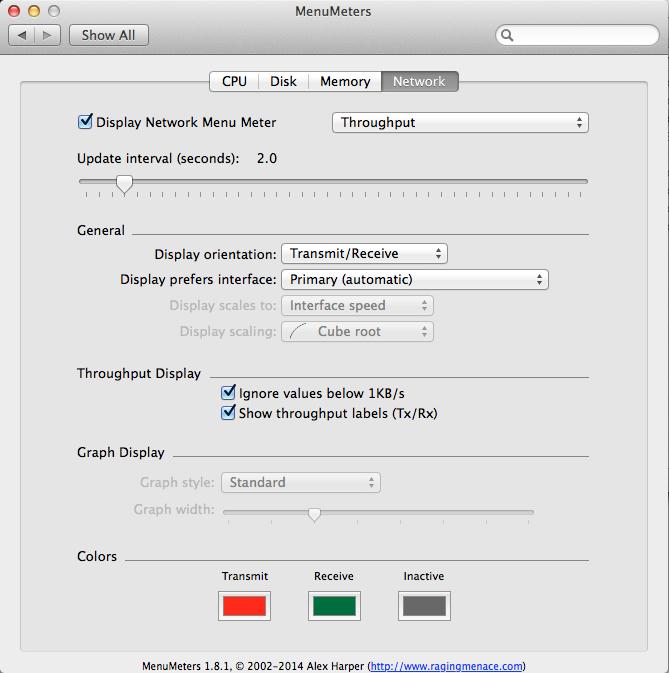
Customizing MenuMeters
MenuMeters is licensed under the GPL and is available to download at www.ragingmenace.com.
Many problems in science and engineering are modeled through ordinary differential equations (ODEs, en.wikipedia.org/wiki/Ordinary_differential_equation). An ODE is an equation that contains a function of one independent variable and its derivatives. This means that practically any system that changes over time can be modeled with an ODE, from celestial mechanics to chemistry reaction rates to ecology and population modeling.
Because of this ubiquity, many tools have been developed through the years to help solve and analyze ODEs. In this article, I take a look at one of the tools available on Linux: Model Builder (model-builder.sourceforge.net). The project is hosted on SourceForge, so you always can build it from source, but most distributions should have a package available. On Debian-based distros, you can install it with the command:
sudo apt-get install model-builder
It also installs several Python modules to support the tasks it can handle. If you do decide to build from source, you will need to handle these dependencies yourself.
Included with the source is a directory of examples. You can use them as a starting point and to gain some ideas of what you can do with Model Builder. Documentation is a bit sparse, so you may need to get your hands a little dirty to take the most advantage of what is possible with Model Builder.
To start Model Builder, you either can click on its menu item in your desktop environment or run the command PyMB from a terminal window. When the main window pops up, you are presented with a template where you can define the problem you are analyzing (Figure 1). The main pane, titled Differential Equations, is where you can define the set of ordinary differential equations that you are trying to solve. The general form of these equations is dy/dt = f(y,t).
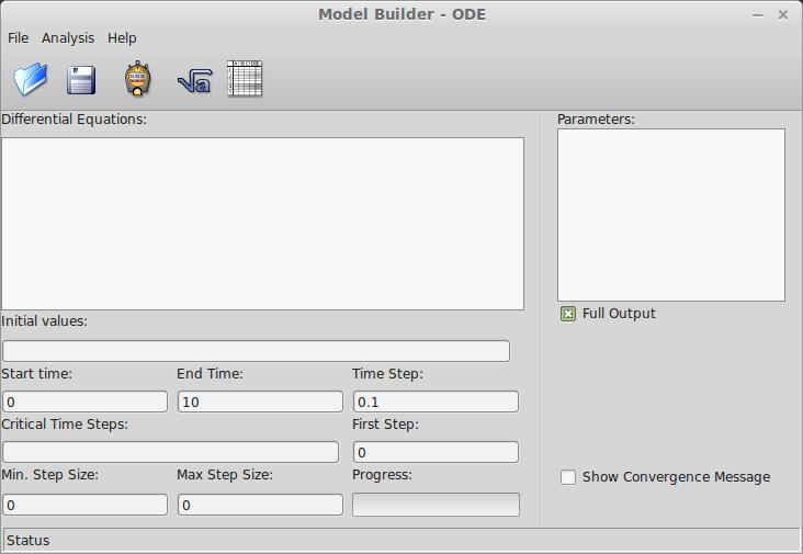
Figure 1. When Model Builder starts, you can set several parameters and the equations you want to analyze.
If your system depends on different levels of differentiating the dependent variable, you always can rewrite it as a system of ODEs. When you give Model Builder your system, you need to write out only the right-hand side of the above equation. This equation can contain essentially any function or expression that NumPy understands, since Model Builder uses Python to do the heavy lifting.
Because Model Builder is designed to handle systems of equations, you need to define the y portion as elements of a list. So the y variable for the first equation is labeled as y[0]; the y variable for the second equation is labeled y[1] and so on. These are called the state variables.
The pane to the right of the equation window is where you can place any parameters that you need, one per line. They can be used in the equation window, where they are labeled as p[0], p[1] and so on. If you want to use time in either the parameters or equations that you have defined, you just need to use the t variable.
Because Python is used in the back end, you even can use lambda functions to define more complex structures. You may want to take a look at the documentation available on the NumPy site to see what options are available (www.numpy.org).
Below these two panes is where you define the rest of the options for your problem. In the Initial values box, you can enter the initial values for each state variable at the time t=0. They need to be separated with a space and put in the order of the equations given in the equation pane.
Below the Initial values, you can enter the start time, the end time and the time step to use in the solution. The critical time steps box is usually left empty, so let's leave it alone here. The first step box is the size of the first step. Usually, you should leave this as 0 to allow for automatic determination. The minimum and maximum step size boxes set these variables that are used in the variable step size algorithm. Typically, you should leave these as 0 as well to allow for automatic determination. The full output check box will print out more useful information about the integration in the results spreadsheet.
Once everything is entered, all you need to do is click the Start icon, and the integration will be calculated. If this is a system that you will want to work with over time, you can click on the menu item File→Save to save the model to a file. This file format is an XML file, so you could edit it with a text editor if you want. When you are ready to do more work with it, you can load it by clicking on File→Open.
Once the calculations are done, which may be fast for simple problems, a results window will pop up (Figure 2). matplotlib handles this graph window, so you can manipulate it just like any other matplotlib window. This includes panning, zooming or changing the plot window. You also can save the resulting plot as an image file in one of several different formats.
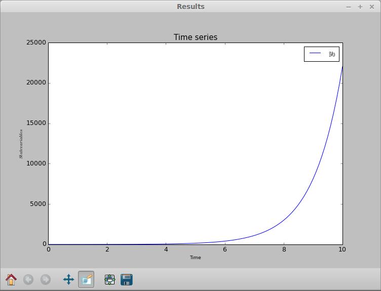
Figure 2. Once you finish defining the problem and run the integration, a result window pops up with a graph of the integration.
Going back to the main window, let's look at some other available tools. Clicking on the Show equations icon pops up a window where you can see the equations typeset (Figure 3). Beside this icon is the Results icon. Clicking on that pops up a spreadsheet of all of the results from your integration (Figure 4). The columns of data include the time, the value of y[0] and the step sizes, among other things. You can select a couple columns by holding down the Ctrl key and clicking on the column headers. Then, click on the plot button to plot them in a new window. You can get a power spectrum for any one column by selecting one of interest and clicking on the Spectrum icon. This pops up two new windows, the first a power spectrum of the column (Figure 5) and the second a spectrogram of the column (Figure 6).
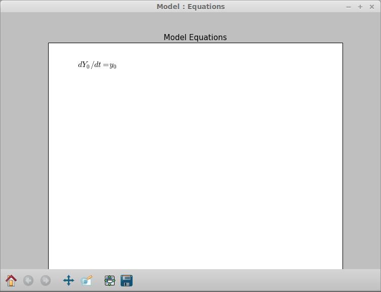
Figure 3. You always can get a typeset display of your equations to verify what they should look like.
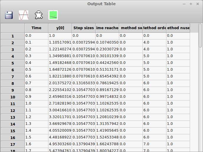
Figure 4. You can pull up all of the results of your integration and do further analysis.
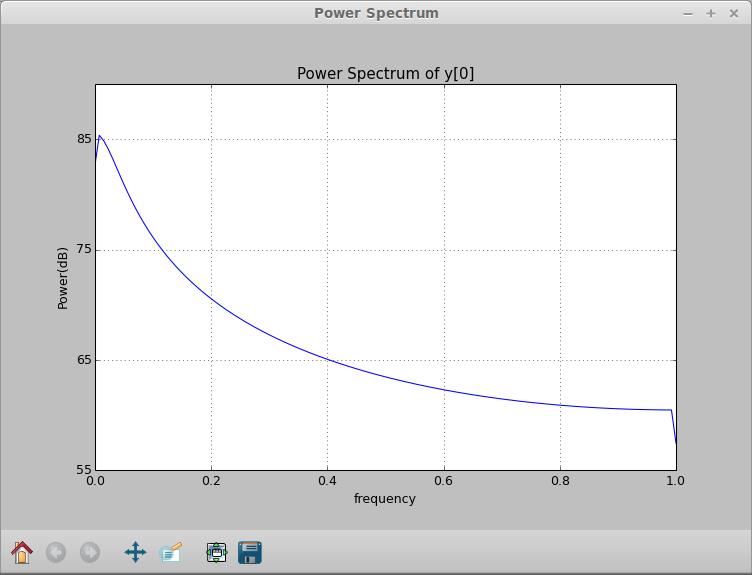
Figure 5. You can generate a power spectrum of any column of your results.
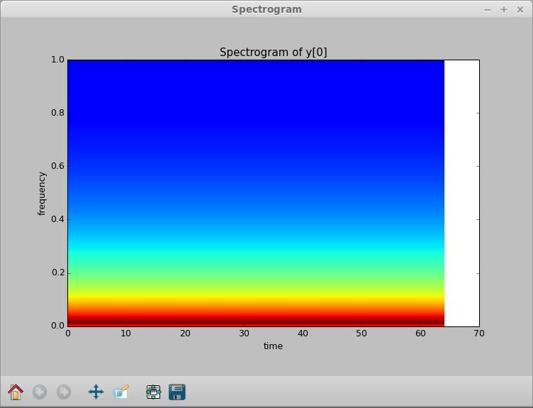
Figure 6. You also can generate a spectrogram of your results.
The last tool available is a wavelet transform. When you select a column, you can apply a continuous wavelet transform to the data. When you are done with Model Builder, you can save this data into a comma-separated values (CSV) file from the spreadsheet window. Then, you can import it into other tools, like R, to do even further analysis.
Now that you have seen the options available in Model Builder, hopefully you will consider it when looking at ODE problems. It provides a pretty simple interface to the tools available in Python to solve ODEs numerically. Although other more powerful tools are available, Model Builder fits into the niche of experimenting quickly with different equations and playing with ideas.
If SSH is the Swiss Army knife of the system administration world, Nmap is a box of dynamite. It's really easy to misuse dynamite and blow your foot off, but it's also a very powerful tool that can do jobs that are impossible without it.
When most people think of Nmap, they think of scanning servers, looking for open ports to attack. Through the years, however, that same ability is incredibly useful when you're in charge of the server or computer in question. Whether you're trying to figure out what kind of server is using a specific IP address in your network or trying to lock down a new NAS device, scanning networks is incredibly useful.
Figure 1 shows a network scan of my QNAP NAS. The only thing I use the unit for is NFS and SMB file sharing, but as you can tell, it has a ton of ports wide open. Without Nmap, it would be difficult to figure out what the machine was running.
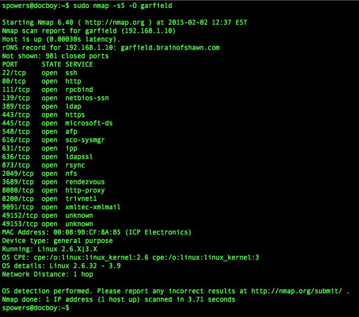
Figure 1. Network Scan
Another incredibly useful way to use Nmap is to scan a network. You don't even have to have root access for that, and it's as simple as specifying the network block you want to scan. For example, typing:
nmap 192.168.1.0/24
will scan the entire range of 254 possible IP addresses on my local network and let me know which are pingable, along with which ports are open. If you've just plugged in a new piece of hardware, but don't know what IP address it grabbed via DHCP, Nmap is priceless. For example, the above command revealed this on my network:
Nmap scan report for
 ↪TIVO-8480001903CCDDB.brainofshawn.com (192.168.1.220)
Host is up (0.0083s latency).
Not shown: 995 filtered ports
PORT     STATE  SERVICE
80/tcp   open   http
443/tcp  open   https
2190/tcp open   tivoconnect
2191/tcp open   tvbus
9080/tcp closed glrpc
This not only tells me the address of my new Tivo unit, but it also shows me what ports it has open. Thanks to its reliability, usability and borderline black hat abilities, Nmap gets this month's Editors' Choice award. It's not a new program, but if you're a Linux user, you should be using it!
SSH is a Swiss Army knife and Hogwart's magic wand all rolled into one simple command-line tool. As often as we use it, we sometimes forget that even our encrypted friend can be secured more than it is by default. For a full list of options to turn on and off, simply type man sshd_config to read the man page for the configuration file.
As an example, one of the first things I do is disable root login via SSH. If you open /etc/ssh/sshd_config as root, search for a line mentioning PermitRootLogin and change it to no. If you can't find a line with that option, just add it to the end. It will end up looking like:
PermitRootLogin no
Plenty of other security options are available as well. Disabling the old SSH version 1 protocol is as simple as changing (or adding):
Protocol 2, 1
Change it to:
Protocol 2
Then only the far more secure version 2 protocol will be able to connect. Every server situation has different security needs. Reading through the man page might reveal some options you never even considered before. (Note that the sshd dæmon will need to be restarted for the changes to be applied. Or, if in doubt, just reboot the computer.)
Do something every day that you don't want to do; this is the golden rule for acquiring the habit of doing your duty without pain.
—Mark Twain
It's okay if you mess up. You should give yourself a break.
—Billy Joel
Let me tell you the secret that has led me to my goal. My strength lies solely in my tenacity.
—Louis Pasteur
If you limit your choices only to what seems possible or reasonable, you disconnect yourself from what you truly want, and all that is left is a compromise.
—Robert Fritz
The highest result of education is tolerance.
—Helen Keller
