
Get to know the language and tools that can take your network filtering rules to a whole new level.
Network filtering is probably as old as networks themselves. If you exchange data with the outside world, it's natural to control what's going in and out. If, however, you capture packets for a good reason (like traffic analysis or intrusion detection), filtering those you are not interested in as early as possible is crucial for performance. The first type of filtering is typically done with a firewall. Berkeley Packet Filter (BPF) is what comes to the rescue in the second case.
Originally, BPF referred to both the capturing technology and its high-performance filtering capabilities. For some Unices (for instance, FreeBSD), this still holds true, and there is a /dev/bpf device from which you can read captured packets. For others, BPF means what it says (the filter), and in this reincarnation, you can find it in various operating systems, including Linux, and with WinPcap and even Microsoft Windows.
BPF filters are programs written in a low-level language similar to assembler (I take a look at that in the last section of this article). These programs are executed by a BPF virtual machine. Most often, this virtual machine resides in the kernel and uses Just-In-Time compilation (JIT) to boost filtering performance. However, user-mode BPF interpreters (useful for debugging purposes or as fallbacks) are available as well—for instance, the one provided with the ubiquitous libpcap library (www.tcpdump.org), the main workhorse behind tcpdump, Wireshark and other popular network tools.
All of this may sound like you need to delve into registers and opcodes just to say you are interested in the packets coming to host 192.168.1.1. Luckily, that's not the case. Of course, if you want (or need) to, you can, but libpcap provides its own high-level filter language that compiles directly to BPF. Largely, this syntax is synonymous with BPF (they are tightly related albeit different things), so I use these terms interchangeably here.
In this article, you'll learn the basics of BPF syntax and also see how it works under the hood.
To get a better idea of what BPF really is, let's go through a set of examples, generating series of packets each time and filtering them as as needed. Sometimes these packets will come from a real network application, but other times you will craft them manually. It's not the best idea to allow these forged packets out from the local host, especially if you are on the office network. So the first step will be to create a virtual Ethernet interface.
Linux already has a concept of “dummy” network interfaces, and the kernel module named dummy implements them. Load it, and assign the dummy0 interface a unique IP address:
# modprobe dummy
# ip link set up dev dummy0
# ip addr add 192.168.2.1/24 dev dummy0
Next, you'll need something to craft the packets and capture them subject to BPF filters. An obvious choice here is Scapy (www.secdev.org/projects/scapy), a Python toolkit for packet manipulation. Install it with your package manager or from the sources. Raw packet generation and live traffic capture are considered privileged operations in Linux, so you'll need to run Scapy as root (for example, with sudo).
Scapy provides an interactive shell (which is naturally Python-based). You create different protocol layers as instances of the classes like TCP, IP or Ether. A complete list is available with the ls() command, and you can add your own protocol if you really want to. The attributes of these classes correspond to protocol fields (addresses, ports, flags and so on). You can use raw numbers (say, 20) or symbolic names (ftp_data) for attribute values. To assemble the packet, use the / Python operator:
>>> Ether(src='08:60:6e:da:31:ae', dst='42:7f:79:88:de:3d') /
 ↪IP(src='192.168.1.5', dst='192.168.2.1')
<Ether  dst=42:7f:79:88:de:3d src=08:60:6e:da:31:ae type=IPv4
 ↪|<IP  src=192.168.1.5 dst=192.168.2.1 |>>
Protocol fields usually have sensible default values (you can check them with ls(IP) or similar), so you need to specify only those you want to override.
To disassemble the packet and get a specific protocol layer, use the [] operator:
>>> _[IP]
<IP  src=192.168.1.5 dst=192.168.2.1 |>
A special _ variable contains the last expression's value. Scapy makes it easy to generate a series of packets that follow a specific pattern:
>>> packets = Ether(src='08:60:6e:da:31:ae',
 ↪dst='42:7f:79:88:de:3d') / IP(src='192.168.1.5',
 ↪dst='192.168.2.1-3') / UDP(dport=[135,(137,139)])
>>> len(list(packets))
12
Here, Scapy crafts 12 packets targeting UDP ports 135, 137, 138 and 139 (common Windows stuff) on three hosts. You can define address ranges with an asterisk (dst='192.168.*.2'), or whole subnets with CIDR notation (dst='192.168.2.0/24').
Several functions send packets over the wire, but here, let's deal with send() and sendp(). The main difference is that sendp() works on Layer 2, so the packet you pass it must have an Ethernet header. send() is for Layer 3, and it looks up the host's routing table to decide what to do with the packet you gave it:
>>> sendp(packets, iface='dummy0')
............
Sent 12 packets.
This way, you push crafted packets into the dummy0 interface.
To capture packets, use the sniff() function. It has many different options, but on these pages, you'll mainly call it like this:
>>> sniff(iface='dummy0', filter='udp')
^C<Sniffed: TCP:0 UDP:12 ICMP:0 Other:0>
>>> _.summary()
Ether / IP / UDP 192.168.1.5:domain > 192.168.2.1:epmap
Ether / IP / UDP 192.168.1.5:domain > 192.168.2.1:netbios_ns
... 10 lines skipped ...
If you omit the iface=, Scapy will listen on all network interfaces. You also can add the count= argument to capture only as many packets as specified; otherwise, you should stop the capture manually with Ctrl-C. Without the filter=, sniff() captures all packets. Internally, Scapy uses libpcap to compile the filter (either directly or via the tcpdump -ddd command), so the syntax is just what you want.
This was a quick tour of Scapy; however, this tool can do much more than you've seen so far. Consult the official documentation (www.secdev.org/projects/scapy/doc) for more information. Or, have a look at Security Power Tools published by O'Reilly (2007), which has a complete chapter (number 6) on Scapy written by its author, Philippe Biondi.
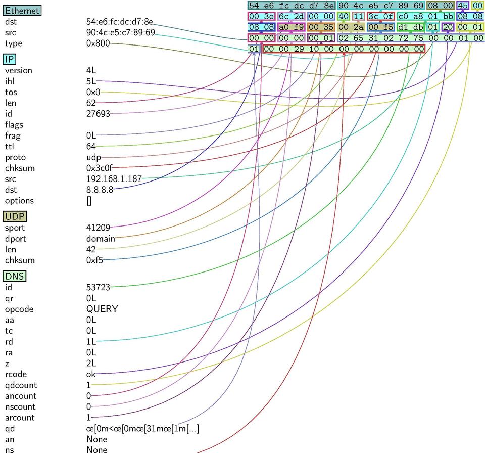
Figure 1. Scapy is a real Swiss army knife. It even can dump packets to PS or PDF.
Now with the tools to experiment with in place, it's time to learn some actual high-level BPF. The most authoritative (and complete) reference documentation is the tcpdump(1) man page. Let's do a quick summary: filter expressions contain one or more primitives combined with the “and”, “or” and “not” keywords (equivalently written as &&, || and !). All basic arithmetic and bit operations are supported as well, and the explicit precedence can be set using parentheses. If you omit parentheses, && and || are of the same precedence, and ! is applied first. Arithmetic and bit operations follow common rules.
Each primitive consists of the ID (either name or number) preceded with an optional protocol (ether, ip, tcp or udp, to name a few), direction (src, dst, src or dst, and src and dst; it is always a single token, so or and and aren't operators) and type (host, net, port or portrange). If some of these are missing, all protocols match; host is assumed for the type, and src or dst for the direction (this means either direction is okay).
The following are valid primitives: udp (no ID here), port 80 (TCP or UDP port 80), ip host pluto (all IP packets for the host “pluto”; the name must be resolvable), dst tcp portrange 0-1023 (packets targeting all privileged TCP ports).
That's enough theory—now let's play. Arguably the most common case is to filter packets by their source or destination IP addresses. Let's use one Scapy instance to generate empty IP datagrams for random (and even nonexistent) hosts:
>>> while True: sendp(Ether(src=RandMAC(), dst=RandMAC()) /
 ↪IP(src=RandIP(), dst=RandIP()) / ICMP(), iface='dummy0')
There are many Rand*() functions in Scapy; two of them are used here.
A second Scapy instance will capture the datagrams that happen to be for host 192.168.1.1 or 192.168.1.2 (note that for the second operand in the expression, the host keyword is implicit):
>>> sniff(iface='dummy0', filter='host 192.168.1.1 or
 ↪192.168.1.2', count=1)
Unless you are very lucky, sniff() will hang until you press Ctrl-C. That's because the probability for a given two addresses to occur in a randomly generated packet series is around 0.0000001%. Let's increase your chances and look for a whole A-class subnet:
>>> sniff(iface='dummy0', filter='net 1.0.0.0/8', count=1)
Equivalently, you can rewrite the filter as net 1.0.0.0 mask 255.0.0.0. This time, sniff() should catch a packet much sooner:
>>> _.summary()
Ether / 185.0.19.206 > 1.205.135.116 hopopt
It's equally easy to filter traffic on ports. For instance, this is a very simple filter for MySQL client-server sessions:
>>> sniff(iface='lo', filter='tcp port 3306')
Try to connect to the MySQL server with the mysql -h 127.0.0.1 -P 3306 command, and you'll see some packets captured. It doesn't matter if the server is actually running—if it doesn't, you'll catch a pair of TCP SYN and RST-ACK indicating the port is unavailable:
>>> _.summary()
Ether / IP / TCP 127.0.0.1:57485 > 127.0.0.1:mysql S
Ether / IP / TCP 127.0.0.1:mysql > 127.0.0.1:57485 RA
Detecting services by the port numbers they use isn't really accurate. Let's do a deeper packet analysis. Imagine you need to collect data pertaining to NTP activity on the local network. NTP messages are sent to (or from, or both) UDP port 123. Moreover, they are 48 bytes in size and have the status of a local clock, which can't be greater than 4, encoded in bits 2–7 of the first octet (see Appendix B in RFC 958 at tools.ietf.org/html/rfc958). Given all of that, the filter you construct will consist of three primitives: udp port 123 (for the first two conditions), and the other two checking the UDP payload length and the clock status value.
To implement them, let's peek inside a protocol payload. BPF uses the [offset:size] operator for this purpose. Offset is measured from byte 0, so for instance, tcp[0] gives the first byte of the TCP header (not a payload). The UDP datagram Length field is at offset 4 and is 16 bits wide. Thus, to check the packet length, you can use the following primitive: udp[4:2] == 48+8 (UDP header length 8 is bytes, and they are included in the Length field as well). The clock status check is a bit more convoluted, but the combined filter looks like this:
>>> ntp = sniff(filter='proto udp and port 123
 ↪and udp[4:2] == 48+8 and ((udp[8] & 0x38) >> 3) <= 4')
Note the operators and hex numbers used—BPF is much like C in this sense. Leave this alone for some minutes, and on a modern Linux distribution you'll sooner or later spot the NTP requests the system sends (and the replies it receives):
>> ntp.summary()
Ether / IP / UDP / NTP v4, client
Ether / IP / UDP / NTP v4, server
...
>> ntp[0][NTP]
<NTP  leap=nowarning version=4L mode=client stratum=2L
 ↪poll=10L precision=233L delay=0.0422210693359
 ↪dispersion=0.0782623291016 id=194.190.168.1 ref=Tue,
 ↪15 Apr 2014 10:00:26 +0000 orig=Tue, 15 Apr 2014
 ↪10:15:20 +0000 recv=Tue, 15 Apr 2014 10:15:20
 ↪+0000 sent=Tue, 15 Apr 2014 10:33:04 +0000 |>
In fact, it works so well, you even can drop the udp proto 123 part without introducing too much error (my quick tests show about a 1% rate).
Another way to get the packet length is to use the len operator. However, it accounts for all protocols used down to Layer 2. So, assuming UDP datagrams are encapsulated in IPv4 with no options and untagged Ethernet frames, you can rewrite udp[4:2] == 48+8 as len == 14+20+8+48. By the way, you also can select packets longer (or shorter) than a specific threshold with the greater and less keywords.
Now you've seen that Scapy can decode (and encode) some application-level protocols like NTP (or DNS). But it can dig even deeper, so for the next example, let's use it to forge VLAN-tagged traffic:
>>> sendp(Ether(src=RandMAC(), dst=RandMAC()) /
 ↪Dot1Q(vlan=[(1,5)]) / 'Nothing to see here', iface='dummy0')
This generates five 802.1Q Ethernet frames with arbitrary MAC addresses and VLAN tags in range 1–5 (note the syntax). Let's not worry about the payload now, so instead of IPv4 (or any other network-level) packet, let's just put raw bytes that form a 'Nothing to see here' string inside the frame.
This is how you can filter traffic with specific VLAN tags in BPF:
>>> sniff(iface='dummy0', filter='vlan 1', count=1)
<Sniffed: TCP:0 UDP:0 ICMP:0 Other:1>
>>> _
<Ether  dst=29:a0:ea:e9:df:ce src=c3:33:a3:9c:63:9c
 ↪type=n_802_1Q |<Dot1Q  prio=0L id=0L vlan=1L
 ↪type=0x0 |<Padding  load='Nothing to see here' |>>>
If you just want to filter out untagged traffic, use filter='vlan'.
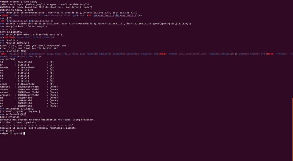
Figure 2. Capture, craft, dissect and do other funky things with network packets in Scapy.
As you already know, BPF filters are actually expressed in a low-level assembler-like language. It targets a register-based virtual machine that has an accumulator register and an index register, along with some memory store. This machine has access to the packet buffer and supports several dozens of instructions that store and load values to the registers or memory, perform arithmetic or logical operations and do flow control. I won't discuss them in detail, but if you want a taste of what they look like, here is the equivalent of a libpcap-compiled simple filter, ip:
ldh [12]
jeq #0x800, Keep, Drop
Keep: ret #0xffff
Drop: ret #0x0000
Opcode mnemonics come from the original BPF USENIX paper (Steven McCanne and Van Jacobson's “The BSD Packet Filter: A New Architecture for User-level Packet Capture” available at https://www.usenix.org/legacy/publications/library/proceedings/sd93/mccanne.pdf). This program loads 16-bit (short) integer (“h” stands for “half-word”) at the fixed offset in the packet buffer (12, the Ethernet Type field) and compares it to 0x800 (the IPv4 protocol number). The filter returns the number of bytes in the packet to allow. Thus, zero means the packet should be dropped, and 0xffff (the maximum possible length) means to accept it entirely.
Linux's own implementation of BPF design is known as Linux Socket Filtering (LSF). It differs from the original BPF slightly (mainly in areas I haven't mentioned in this article), but largely what I've said here about BPF applies to LSF.
Given that the virtual machine is register-based, it comes as no surprise that its bytecode easily can be compiled to real machine instructions. It is exactly what a BPF JIT compiler (introduced in Linux 3.0) does. On my x86_64 system, the code above compiles into:
 0:   push   %rbp
 1:   mov    %rsp,%rbp
 4:   sub    $0x60,%rsp
 8:   mov    %rbx,-0x8(%rbp)
 c:   mov    0x68(%rdi),%r9d
10:   sub    0x6c(%rdi),%r9d
14:   mov    0xd8(%rdi),%r8
1b:   mov    $0xc,%esi
20:   callq  0xffffffffe104b2b3
25:   cmp    $0x800,%eax
2a:   jne    0x0000000000000033
2c:   mov    $0xffff,%eax
31:   jmp    0x0000000000000035
33:   xor    %eax,%eax
35:   leaveq
36:   retq
This is a small function. By convention, the return value is stored in %eax register. Everything up to offset 0x1b is the utility stuff, but you easily can spot loading 0xc (12) to %esi (x86 source index register) and compare the result to 0x800. A few dozens of machine-level instructions are needed to check the filter against a packet, and since BPF was designed to execute filters on the original packet and not a copy of it, this should really be a fast process.
To control BPF JIT in the Linux kernel, you write to /proc/sys/net/core/bpf_jit_enable (or use the corresponding sysctl—see Jonathan Corbet's “A JIT for packet filters” at https://lwn.net/Articles/437981). A value of 1 means to enable JIT, and a value of 2 means to enable tracing. When tracing is enabled, JIT code for the filter is printed to the kernel log buffer (that's what dmesg reads). With this in place, you can use the bpf_disasm tool (it comes with the Linux kernel sources) to print a disassembly.
With the neat high-level language libpcap provides, it is unlikely you will need to program in BPF “assembler” directly. But if you ever want some BPF feature that libpcap doesn't provide (maybe filtering by Netfilter mark value or something else Linux-specific), take a look at netsniff-ng (netsniff-ng.org). This toolkit contains a fully functional BPF compiler, bpfc.
Finally, what if you want to integrate BPF filtering capabilities into your own code? If it isn't possible (or feasible) to link against libpcap (or use one of its bindings), you can call the native kernel interface directly. BPF filter programs are represented as struct sock_fprog that has a pointer to the array of opcodes (struct sock_filter *) and a program length field. A sock_filter structure is what tcpdump -dd (or bpfc) prints for you:
# tcpdump -i dummy0 -dd ip
{ 0x28, 0, 0, 0x0000000c },
{ 0x15, 0, 1, 0x00000800 },
{ 0x6, 0, 0, 0x0000ffff },
{ 0x6, 0, 0, 0x00000000 },
Sometimes (for example, in a script) you even can execute this command in the runtime (it is exactly what Scapy does when conf.use_pcap is False).
Filters are attached to (and detached from) the socket with the setsockopt(2) system call:
setsockopt(sockfd, SOL_SOCKET, SO_ATTACH_FILTER,
 ↪&bpf, sizeof(bpf));
Here, sockfd is the socket descriptor and bpf is the struct sock_fprog.
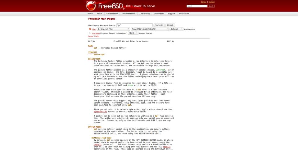
Figure 3. BPF and LSF are not the same; however, you still can use BSD-originated man pages.
So far, I've spoken of BPF (and LSF) as a socket-level facility. To conclude this article, let's look at it from a different angle. Starting with Linux 3.9, there is an xt_bpf module that allows you to use BPF in xtables rules:
iptables -A INPUT -m bpf --bytecode "$(nfbpf_compile
 ↪RAW 'tcp dst port telnet')" -j DROP
The nfbpf_compile utility comes with iptables, provided those were built with the --enable-bpf-compiler flag to the configure script.
Some tests show that xt_bpf performs even faster than the u32 xtables module, so it's worth considering when you optimize your firewall rules.
Berkeley Packet Filters and their OS-specific implementations are no substitute for conventional firewalling code (like Netfilter in Linux). However, they may become indispensable when a fast application or system-level traffic filtering is the requirement.
