
Extend PostgreSQL's capabilities with PostGIS 2.0 and discover all the magic of spatial databases.
Even if you're unfamiliar with GIS, I am pretty sure you know what Web mapping is. GIS stands for geographical information systems, and it originated in the early 1970s as a set of tools and techniques for scientists (cartographers, land planners and biologists). Since then, the field has been experiencing an amazing evolution, as in many other computer-related fields. One of the most revolutionary things is that now maps, and especially Web mapping, are a common experience for millions of people in everyday life. Not only in the past few years have we seen people using more and more mapping apps, there has been an explosion in personal Web mapping. Today, a lot of blogs and personal Web sites have maps.
So, what's special with spatial data? Not really very much—a lot of data has location references (think of your address book as a trivial example), but the spatial component is not really organized. When you want to organize your spatial data, you need to do it with the proper tools.
Spatial data, as all other data types, needs to be stored somewhere. An RDBMS is a great tool for storing, processing and analyzing huge amounts of data, but you will need an RDBMS with a spatial extension if you are going to go this route. Do you know a great open-source RDBMS? I bet you do. Many of us commonly use MySQL in Web applications, but when it comes to spatial data, it's not the first choice. Your friend when it comes to spatial data is PostGIS, an amazing companion of PostgreSQL.
I'm sure you've heard of PostgreSQL. It's probably the most famous open-source RDBMS, and LJ has covered it often in the past. If you're not familiar with it though, check out Reuven M. Lerner's “PostgreSQL 9.0” in the April 2011 issue of LJ (www.linuxjournal.com/article/10986).
PostGIS is not a new project. It started in 2001 and reached maturity at release 1.0 in 2006. On April 3, 2012, 2.0 was released. Version 2.0 is a major shift, and it indeed broke backward compatibility. PostGIS developers were forced to cause this break because of a new serialization (see Resources). On June 22, 2012, version 2.0.1 was released, a bug-fixing release, and this is the latest release at the time of this writing.
Whether or not you have PostgreSQL installed on your Linux box, getting PostGIS up and running is really simple. You can download the source code and compile it yourself, which isn't hard, but it's not really necessary for a first look at PostGIS. If you love compiling, take a look at the reference material—the official documentation is very detailed and complete. There also are lots of blog posts from the community about custom installations.
When you have no specific requirements, the easy way often is the best. You can use the package delivered by your Linux distribution (for example, type sudo apt-get install postgresql-9.1-postgis for Debian distributions). However, as with other rapidly evolving software, you are not going to find the latest release.
A binary prepared by EnterpriseDB may come in handy if you want the bleeding-edge version. Installation is really straightforward, and it also includes Stack Builder, a utility to add tools and upgrade your installation with future releases.
Being an extension of PostgreSQL, you may wonder what PostGIS adds to the many functions shipped with PostgreSQL. In a nutshell, it extends storage, retrieval and analysis capabilities of spatial objects. Let's look at an example to better explain how it works. You know an RDBMS can answer questions like “How many employers are currently on holiday in each department?”. The standard way to ask it with PostgreSQL is by speaking SQL:
SELECT COUNT(E.SERIAL) AS #, D.NAME FROM EMPLOYERS E
 ↪JOIN DEPARTMENT D ON (DEP_ID)  WHERE E.ON_HOLYDAY = 1
 ↪GROUP BY D.NAME ORDER BY D.NAME
What if your question has a spatial component? Suppose you want know how many houses are within 3 kilometers from the new highway path in your county. Standard SQL has no features to express this, but here comes PostGIS to help perform the analysis:
SELECT COUNT(id) FROM houses WHERE ST_DWithin(geom,(SELECT
 ↪highway.geom FROM county, highway WHERE ST_Intersects
 ↪(county.geom, highway.geom) AND county.name = 'Orange'
 ↪AND highway.name = 'Interstate 5'),3000);
Does it seem powerful? Indeed it is! The code fragment above should give you some hints about what PostGIS provides—a huge set of special functions, prefixed with ST_ for querying and processing, plus two new data types called geometry and geography.
Of course, geometry and geography are the data types for spatial features. They are quite similar. Both let you store simple geometrical objects in a table. The big difference is that geography accepts geodetic coordinates (that is, expressed in degrees on a spherical reference system), while geometry accepts coordinates defined over a planar reference system. Geography was introduced in PostGIS with release 1.5.0, and due to underlying complex math, only a few functions support it.
The simple features I'm talking about are points, lines and polygons. With them, you can model the true world. Indeed, this is a standard approach—the simple features' properties and behaviors were modeled by the Open Geospatial Consortium (OGC, an organization committed to defining open standards for GIS and data interoperability), and PostGIS, since its early versions, was built with a strong support for that standard.
Adding geometry support to a table is really simple. Suppose you are building a table of world capitals, you would start with basic properties:
CREATE TABLE capitals (
id SERIAL,
state_name TEXT,
capital_name TEXT,
population numeric(8,0),
PRIMARY KEY(id)
);
If you are going to store features that can be represented on a map, you need to add a spatial reference. Point geometry may be a good approach; AddGeometryColumn is the function you need:
SELECT AddGeometryColumn('gisuser',
 ↪'capitals','geom',4326,'POINT',2);
Here, you passed values for schema, table name, geometry column name, spatial reference system and geometry type. The last value means you want a two-dimensional geometry (that is, a point defined on a surface). If you are going to store elevation, you can set three as the dimension value. And there's more. PostGIS also supports four-dimensional geometry. Well, the fourth dimension is not for travel trips, but it is useful to associate a measure to the geometry, and the fourth dimension is indeed called M. For example, a stream network may be modeled as a multilinestring value with the M coordinate values measuring the distance from the mouth of stream. The method ST_LocateBetween may be used to find all the parts of the stream that are between, for example, 10 and 12 kilometers from the mouth.
Before using your table, it is better to create an index on the geometry column. The syntax is equivalent to any other index creation; the index type is GiST (Generalized Search Tree) somewhat similar to an R-Tree index:
CREATE INDEX capitals_geom_gist ON capitals USING gist (geom);
Now let's add real data to the table. How do you insert values in the geometry column? The ST_GeomFromText function translates numeric values for you. So let's insert the coordinates you picked up in London when you were watching the Olympic games:
INSERT INTO capitals (state_name, capital_name, population, geom)
 ↪values('UK','London', 6500000,
 ↪ST_GeomFromText('POINT(-0.01639, 51.53861)', 4326));
The text you are passing to the function is called a Well-Known Text (WKT) representation of spatial objects. Points are really simple to define, but how do you express a line or a polygon? You could mimic the capitals table definition to create a rivers table and add a record for the Thames:
ST_GeomFromText('LINESTRING(0.31221 51.47033, 0.33477 51.45171,
 ↪0.44437 51.45851, 0.45877 51.48934, 0.61523 51.49512)',4326)
Another table could contain famous buildings represented by polygons. You can find Westminster Abbey here:
ST_GeomFromText('POLYGON((-0.12850 51.49963, -0.12856 51.49929,
 ↪-0.12814 51.49927, -0.12822 51.49896, -0.12722 51.49890,
 ↪-0.12714 51.49919, -0.12627 51.49933, -0.12711 51.49957,
 ↪-0.12707 51.49971, -0.12751 51.49974, -0.12758 51.49956,
 ↪-0.12850 51.49963),(-0.12810 51.49902, -0.12805 51.49924,
 ↪-0.12757 51.49921, -0.12761 51.49897, -0.12810 51.49902))',4326)
The WKT for the polygon contains two coordinate lists enclosed in round parentheses, while lines always are defined by a single list. Indeed, a polygon may contain holes. The first list defines the external ring of the polygon while the following lists, you can have as many as you need, define internal rings that encircle holes.
Knowing that your features are safely stored in a database is nice, but you may want to use them for purposes other than later retrieval. PostGIS functions let you interact with spatial objects and explore their relationships.
Functions known as constructors build geometry from definitions in several formats. They are sort of like translators. You used it before with WKT, and ST_GeomFromKML and ST_GeomFromGeoJSON enable translations from other popular formats. Output functions enable the inverse translation as in ST_AsText, ST_AsGeoJSON and ST_AsKML.
ST_IsValid and ST_GeometryType check fundamental properties of geometry. You can interact with geometry with ST_NumPoint to retrieve the total number of vertexes and ST_PointN to get the nth vertex; ST_RemovePoint removes the vertex at the position you pass to the function. Function names often are self-explanatory, as with ST_Scale and ST_Rotate.
ST_Distance measures the minimum distance between two geometry objects. As others, this function is overloaded, the exact definition is:
float ST_Distance(geometry g1, geometry g2);
float ST_Distance(geography gg1, geography gg2);
float ST_Distance(geography gg1, geography gg2, boolean use_spheroid);
The returned distance is measured along a Cartesian plane for geometry, and along a spheroid/sphere for the geography type. If you are querying objects relatively nearby, the question of how to use them may seem futile, but think about measuring the distance from San Francisco to Denver:
SELECT to_char(round(ST_Distance(
ST_GeomFromText('POINT(-122.440 37.802)',4326)::geography,
St_GeomFromText('POINT(-104.987 39.757)',4326)::geography
)),'999,999,999');
1,529,519
About 1,530 km is quite a long way to go, and going straight from San Francisco to Denver may be a real challenge, so there's room for extra mileage. But if you try to measure the same distance on a printed map, you may find a rather different result. As you learned in primary school, the Earth's shape is almost a sphere. When a map represents a wide portion of the planet on the surface of a plane (yes, curved monitors are yet to come), it has to distort the real shape and distance. By passing two geography objects to ST_Distance, you are asking it to perform a distance calculus over the sphere's surface. Let's use geometry, and it will use a Cartesian plane for the calculus:
SELECT to_char(round(ST_Distance(
ST_Transform(ST_GeomFromText('POINT(-122.440 37.802)',4326),3857),
ST_Transform(ST_GeomFromText('POINT(-104.987 39.757)',4326),3857)
)),'999,999,999');
To get the result in meters, comparable to the previous one, you need to add the ST_Transform function to change on the fly the SRS to the Web Mercator used by most Web mapping systems:
1,962,818
More than 1,900km! Hey, Mr Mercator, where are you taking me?
You've learned how you can process spatial data in many ways inside PostGIS, but how do you get the data into the database? If you are familiar with PostgreSQL, you know it is shipped with psql, a command-line tool, or you probably have been using pgAdmin III if you prefer to interact with a GUI. Both are not specialized at dealing with spatial data, but you can execute SQL code that performs data loading.
If you search on the Internet, you quickly will realize that a lot of data is available in shapefiles, a binary proprietary format that is the de facto standard in spatial data exchange. Are you wondering how you can transform the binary format in an SQL script? Don't worry; since its early releases, PostGIS has included some tools that read shapefiles and load them in the database.
shp2pgsql and pgsql2shp are command-line tools that make your data go in and out. Not surprisingly, shp2pgsql loads the data. In fact, shapefiles are not really loaded by shp2pgsql but are translated in a form that psql can keep and load for you. So, you just have to pipe the output to psql:
$ shp2pgsql -s 4269 -g geom -I ~/data/counties.shp
 ↪public.counties | psql -h localhost -p 5432 -d
 ↪postgisDB -U gisuser
The basic set of parameters required are -s to set the spatial reference system, -g to name the geometric column (useful when appending data) and -I to create a spatial index. There are quite a few other parameters that make it a flexible tool. As usual, -? is your friend if you need to execute less-trivial data loading. Apart from creating a new table, the default option, you may append data to an existing table, drop it and re-create or just create an empty table modeling its structure according to the shapefile data. pgsql2shp lets you drop your data in a shapefile:
$ pgsql2shp -f ~/data/rivers -h localhost -p 5432 -u
 ↪postgres postgisDB0 public.rivers
The source of the data can be a table or a view, but you also can filter data at extraction time to export only a portion of a table:
$ pgsql2shp -f ~/data/california_counties -h localhost -p
 ↪5432 -u postgres postgisDB "SELECT * FROM
 ↪public.counties WHERE statefp = '06'"
As declared in its name, shp2pgsql-gui is a graphical version of shp2pgsql. Release 2.0 introduced some interesting features. Despite the name, you now can use it both for loading shapefiles and for exporting them, and although earlier versions processed one shapefile at a time, now you can add as many files as you need to load and then run it once.
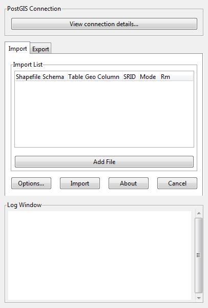
Figure 1. Shapefile Loader GUI
Storing and processing raster data in PostGIS is analogous to vector data. Aerial imagery and satellite scenes, like those visible in Google maps, are common examples, but other types may be way more useful inside PostGIS. Indeed, the real value to having raster data inside PostGIS is the possibility to perform analysis. You also can mix raster and vector data in your analysis. The digital elevation model, a raster where an elevation value is associated to each pixel, is commonly used to perform terrain analysis by geologists. A raster data type has been added to support this kind of data. You can create a table for raster storage in the same way that you did for a vector:
CREATE TABLE myraster(rid integer, rast raster);
A raster is tiled in regular tiles, and each block is loaded as a record in the table. For example, if you have an imagery.tif file whose size is 4096x3072 pixels, and you choose a tile size of 256x256 pixels, after loading it, you will have a table with 192 records.
Loading raster data from the SQL prompt is not easy. As with vectors, a command-line utility exists, raster2pgsql:
$ raster2pgsql -s 4326 -t 256x256 -I -C
 ↪/home/postgis/data/imagery.tif imagery |
 ↪psql -d postgisDB -h localhost -p 5432 -U gisuser
Parameters are very similar except you use -t to set tile sizes, and -C sets the standard set of constraints on the raster.
This article is merely a brief exploration of what PostGIS can do. Consider that there are about 700 specialized functions for dealing with spatial data. I hope you found it interesting and want to give it a try. Among experts, PostGIS always has been considered to be a hard horse to ride. I think it requires a little humility and a willingness to read the manual. Once you start using it, however, you soon will find yourself asking why people are spending big bucks for commercial spatial databases.