
The Rocks clustering package from the University of California at San Diego makes it easy to build and maintain a high-performance compute cluster with off-the-shelf hardware.
You have an application running on a relatively new dual-core workstation. Unfortunately, management wants it either to complete faster or be able to take on a larger dataset in the same time as it runs now. You do a bit of investigating and find that both SMP and cluster versions of the application are available. You are using the SMP version on the workstation. You could speed things up if you could run on a quad core (or more) workstation, but the boss is not too receptive to the expenditure in the current economic climate. But wait, you do have a pile of 32 single-socket servers that were replaced earlier in the year. They're only single core, but 32 of them should have more capacity than the dual-core workstation, if you can just find a way to get them all to play together—that would be a cluster.
So, what is a cluster? Here's one accepted definition: a cluster is a group of computers all working together on the same problem. To accomplish this, the machines in the cluster must be appropriately interconnected (a network) and trust each other.
It is possible to configure the networking and security manually, but there are easier ways to accomplish this using any one of a number of cluster provisioning and management systems. At the moment, one of the more popular packages is the Rocks package maintained by a team at the University of California, San Diego, under a grant from the National Science Foundation.
Rocks is termed a cluster provisioning, management and maintenance package. It helps you set up the cluster in the first place (from bare metal); it provides the tools to run parallel programs, and it provides the tools to maintain and extend the cluster after it is created.
The package is delivered as a series of .iso images that you burn onto a series of CDs or DVDs. You then boot the machine that will become the head node from the appropriate DVD or CD, and the installation routine guides you from there. After asking a minimum number of questions in an interactive phase, the installation program builds the head node. Upon reboot, you invoke a single routine (insert-ethers) to add the rest of the machines as compute nodes. To add a compute node, you simply network boot it, and it will be added to the cluster, loaded and configured automatically. After the last node is complete, you have a functional cluster, ready to execute parallel applications.
So, with all of this in mind, let's build a cluster with those otherwise unloved machines.
The first item on the agenda is setting up the hardware. The overall idea is to have a set of connected computers. Ideally, the machines in the cluster should be as identical as possible, so no single machine or group of machines will be the weak link in any parallel computation. The same homogeneity should apply to the network, because most parallel computation relies on continuous communication between all of the nodes within the cluster.
Find a spot to set up your 32 servers, and make sure you have enough power and cooling to support them. As you connect all of the servers to power, label both ends of each power cord so you can keep track of what is connected to each power strip in the rack.
Because you are starting with a clean sheet, now is a good time to update and configure the BIOS on each system. Set the BIOS clock to the current time as closely as practical (plus or minus five minutes is a good goal). Most clustering packages keep the BIOS clocks synchronized during operation, but only if the clock is reasonably close to the correct time at the beginning.
Because the machines are used, it's prudent to wipe all the disks before loading the cluster software. There are many ways to accomplish this. One fairly thorough method is to use DBAN (Darik's Boot and Nuke). This self-contained application can perform several disk wipe techniques, including two that have some level of Department of Defense approval.
Remember, the goal here is to make all the machines in the cluster as identical as possible. But, this is a goal, not a hard and fast requirement. Heterogeneous clusters will work, but you may need to be careful as to how you deploy workloads on the machines to get the best performance.
Now that you have all the compute nodes configured and in the rack, it's time to set up the communications network. Figure 1 shows a typical networking setup for a simple compute cluster. In this configuration, the Ethernet fabric most likely would be used for administrative purposes, while the InfiniBand fabric would carry the compute traffic. If you don't have InfiniBand hardware available, you can just ignore the bottom section of the diagram. The Ethernet fabric can carry both the administrative and compute traffic.
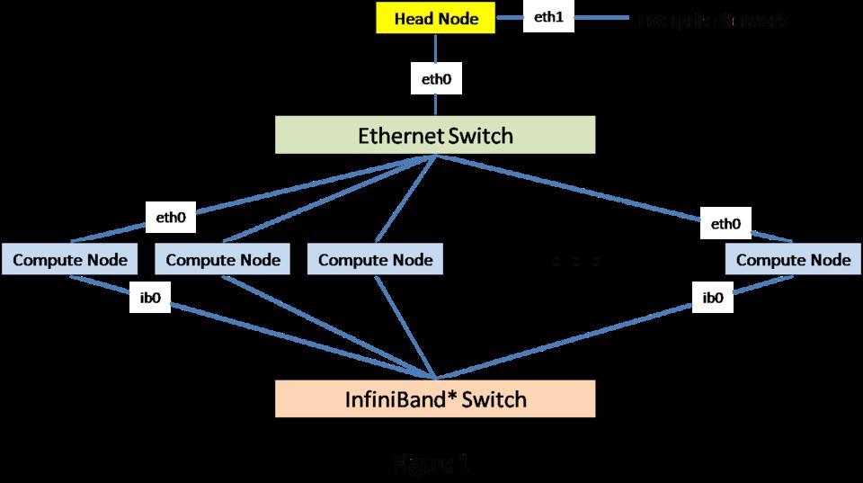
Figure 1. Network Setup for a Compute Cluster
The best Ethernet network configuration for your cluster would be a single 48-port switch. If a switch like that is not available, you always can resort to a set of smaller federated switches forming a full fat tree network for the cluster. Like the compute nodes themselves, the network should be as uniform as possible.
Plan all the cable runs, remembering that Ethernet cables have a nonzero cross section. Before you install them, test each cable. There is nothing as aggravating as finding that a cable is bad after it has been tied into the rack in a dozen places. Once again, label both ends of each cable to make troubleshooting simpler if it is necessary.
Select one machine to be the head node for the cluster. The rest of the machines will be the compute nodes in your new cluster. As it installs the compute nodes, Rocks numbers the machines as compute-x-y, where the x is the rack number, and y is the number of the machine within a rack. Say you spread the 32 nodes over four racks. If you want to follow the Rocks naming convention, you would set things up as follows: rack 0 contains the head node, so the numbering of the nodes would be compute-0-0 to compute-0-6. Rack 1 would come out as compute-1-0 to compute-1-7. Rack 2 would contain compute-2-0 to compute-2-7. Rack 3 would follow suit.
Alternatively, you simply could pretend that all the machines are in a single rack: compute-0-0 to compute-0-30. Either way works, so use whatever is comfortable for you.
First, you need to get a copy of the Rocks package that will be appropriate for your cluster's hardware. Navigate to the Rocks Web site, and select the Download tab at the top of the home page to access the various versions of the package. The 5.1 version is the latest at the time of this writing. Click the link to get a listing of the components of the package. For this exercise, I selected the x86-64 Jumbo DVD image, downloaded it and burned it onto an empty DVD. While you are at the site, download the documentation. If nothing else, it will give you something to read while the software loads.
Boot the head node from the newly minted Rocks DVD. If everything is working as it should, you will be greeted with the welcome screen shown in Figure 2.
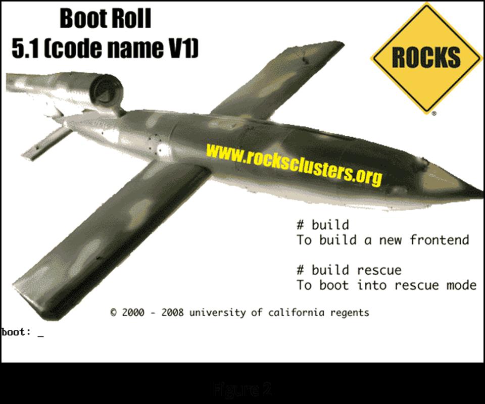
Figure 2. Rocks Welcome Screen
Enter build at the boot: prompt to start the installation sequence. The system boots in the normal Linux fashion and eventually presents the user with the initial Rocks configuration screen shown in Figure 3.
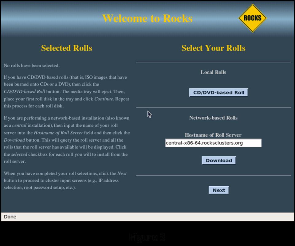
Figure 3. Rocks Configuration Screen
Because you have all of the software components on the Jumbo DVD, you will do your installation from CD/DVD-Based Rolls. Select CD/DVD-Based Roll. This brings up a screen listing all the individual components you can select from the DVD (Figure 4).
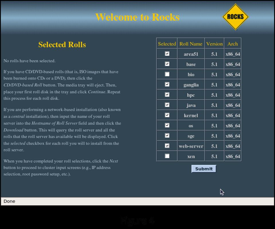
Figure 4. Rolls Selection Screen
For the purposes of this installation, I selected everything except the Bio Roll and the Virtualization Roll. You probably will select a different set of components. At absolute minimum, you need to select the Base, Web Server, Kernel and OS Rolls. Once you have made your selections, click Submit to continue the installation.
The installation now repeats the first screen, showing your selections (Figure 5). If you are satisfied with your selections, click Next to continue to the first of the administrative screens in the installation. If you want to make a change, click CD/DVD-Based Roll to go back to the component selection screen.
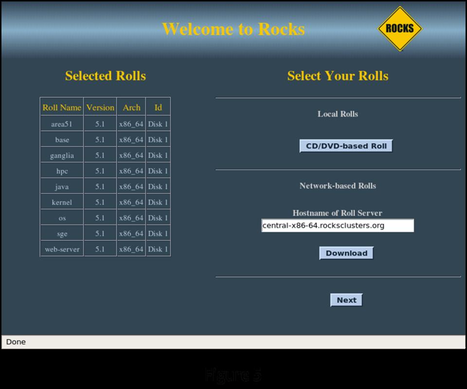
Figure 5. Rolls Selected Items Screen
As you enter data on these screens, the installation routine is building a small MySQL database that details all of the component configurations in your cluster. The various tables Linux needs to run (like /etc/hosts) will be generated as an SQL report from this database. If you want to make changes in the system's configuration, the tools that Rocks provides actually change the database first, then run the appropriate reports to regenerate the system configuration files. This significantly reduces the chance for errors to creep into these files. It still is possible to edit the automatically generated system files manually, but remember that the next time you use the Rocks tools to reconfigure the cluster, your manual changes will be overwritten by the automatically generated SQL report versions.
The next screen (Figure 6) allows you to enter information about your cluster. If the cluster will be connected to your enterprise network, you should enter a fully qualified hostname to be consistent with your domain. The cluster name you enter in the Cluster Name field will appear in the management screens during cluster operation. Once you are satisfied with your entries, click Next to go to the configuration of the head node network connection to the private network (eth0).
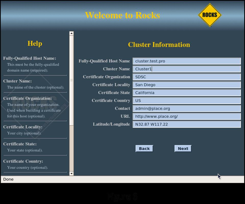
Figure 6. Cluster Information
The next screen (Figure 7) lets you configure the cluster's network. The installation routine automatically selects 10.1.1.1 as the IP address for eth0 on the head node. Because this is a private network, you probably won't need to change this setting. If your public network also happens to be in the 10.1.X.X configuration, change this to something that doesn't conflict with your existing network. Clicking Next brings up the head node public network connection configuration screen.
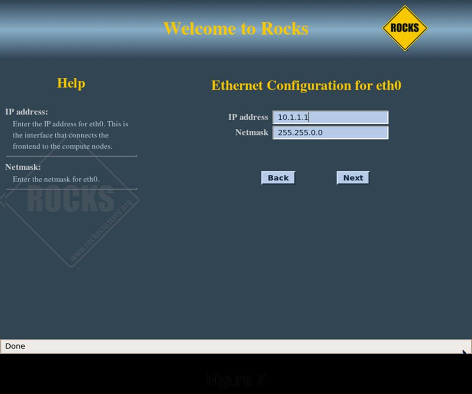
Figure 7. Network Configuration
Figure 8 shows configuring the “public” connection of the head node, its connection to the rest of your systems. The public connection for the head node must be configured with a fixed IP address. The public network for this example is configured as 192.168.0.X with a netmask of 255.255.255.0. Make sure the head node does not conflict with other servers and workstations on the public network. On the following screen (Figure 9), configure the local Gateway and DNS Server IP addresses for the head node to use.
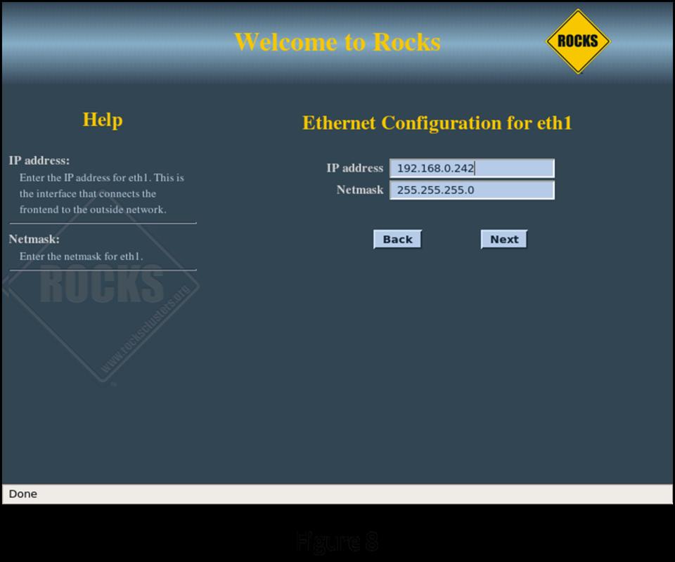
Figure 8. Head Node Public Network Configuration
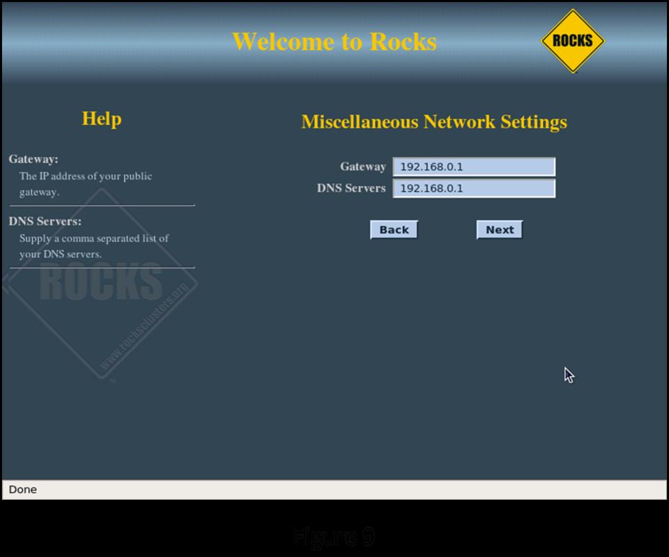
Figure 9. Head Node Gateway and DNS Configuration
On the next two screens (Figures 10 and 11), enter the root password and configure the time zone and NTP server for the head node.
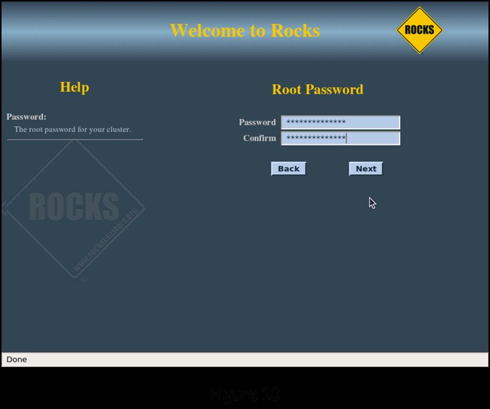
Figure 10. Root Password
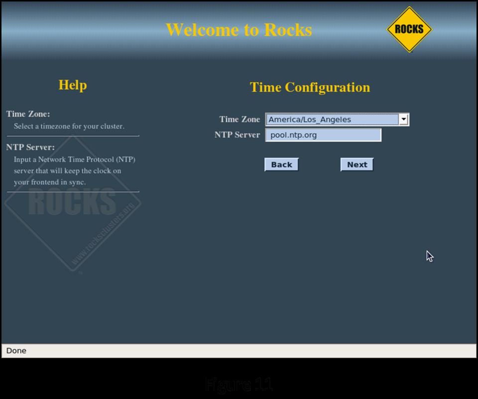
Figure 11. Time Zone and NTP Server
The final interactive screen of the installation sequence (Figure 12) is the disk-partitioning screen. You can partition the disks automatically or manually. If you go with the automatic partitioning scheme, the installation routine sets up the first disk it discovers as follows:
Partition                         Size
/                                 16GB
/var                              4GB
swap                              Equal to RAM size on the head node
/export (aka /state/partition1)   Rest of root disk
If you have multiple disks on the head node or you want to arrange the disk in a different fashion, select Manual Partitioning. This takes you to the standard Red Hat manual partitioning screen where you can configure things any way you desire (you still need to have a 16GB / partition and an /export partition at minimum though). Clicking Next on the disk-partitioning screen begins the automatic portion of the installation (Figures 13, 14 and 15). Once installation is complete, the head node reboots, and you are greeted with your first login screen (Figure 16).
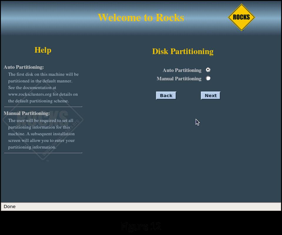
Figure 12. Disk Partitioning
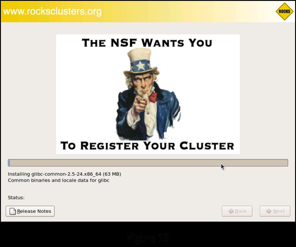
Figure 13. Rocks Installation, 1
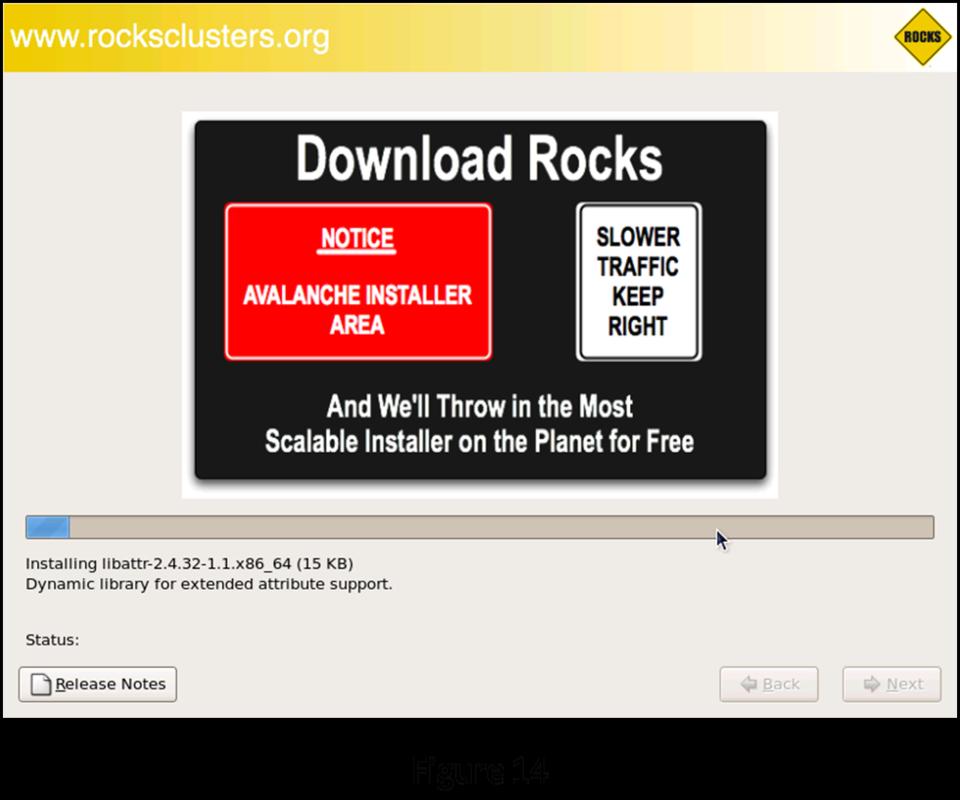
Figure 14. Rocks Installation, 2
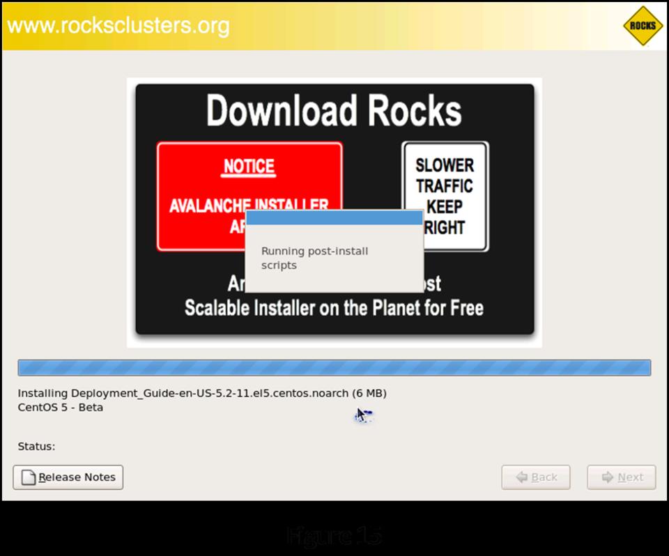
Figure 15. Rocks Installation, 3
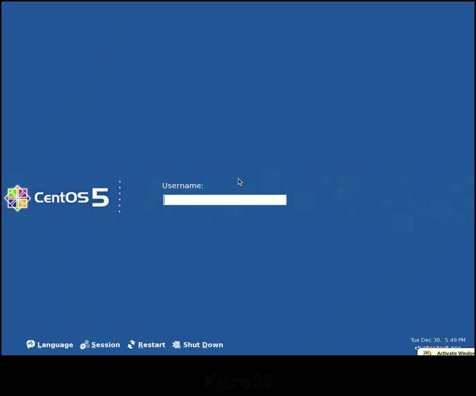
Figure 16. Login Screen
Log on as root, and wait for two or three minutes. This lets the remaining configuration routines finish setting up the cluster in the background. Start a terminal session (Figure 17) to begin installing the compute nodes.
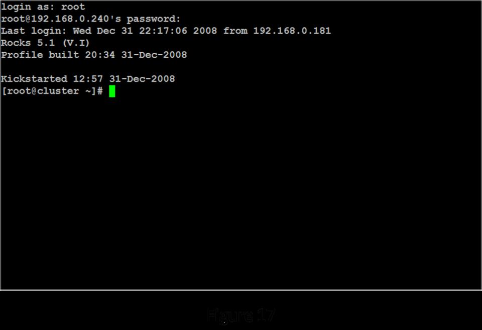
Figure 17. Root Terminal
Now you're ready to add nodes to the cluster. The Rocks command that accomplishes this is insert-ethers. It has quite a few options, but for this example, use the main function of inserting nodes into the cluster. After you invoke insert-ethers, you are presented with the screen shown in Figure 18.
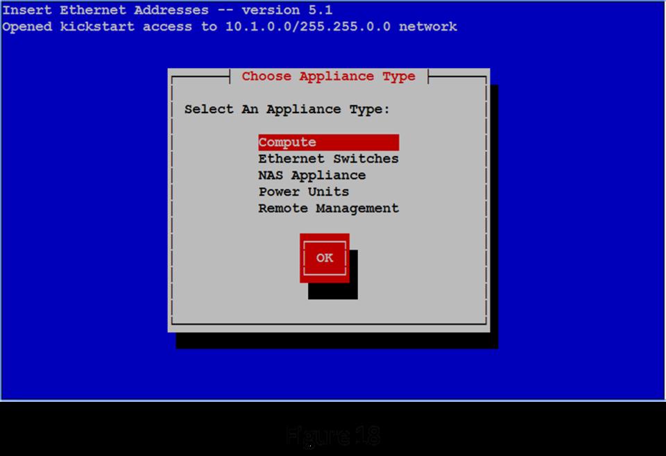
Figure 18. insert-ethers
Rocks treats everything that can be connected to the network as an appliance. If it can respond to a command over the network, it's an appliance. For this simple example with a dumb switch, the only things you need to worry about are the compute nodes themselves. Because Compute is already selected, tab to the OK button and press Enter. This brings up the empty list that will be filled with the names and MAC addresses of the nodes as they are added (Figure 19).
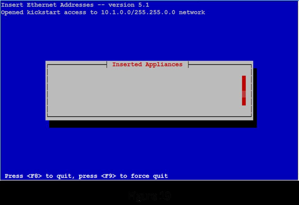
Figure 19. List of Installed Appliances (Empty)
Now it's time to boot the first compute node. If you have wiped the disk, most systems will start a PXE boot from the network as a default action. If you have a KVM switch and can watch the console on the compute node, you should see the PXE boot begin. When the compute node asks for an address for eth0, you will see the MAC address entered in the Inserted Appliances list on the head node (Figure 20).
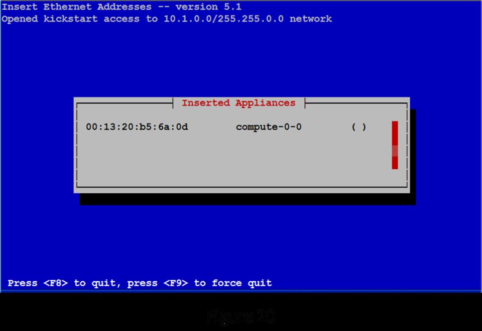
Figure 20. List of Inserted Appliances (First Node Added)
The insert-ethers routine displays the MAC address it has received and the node name it has assigned that node. The ( ) will be filled in with an asterisk (*) when the compute node begins downloading its image (Figure 21).
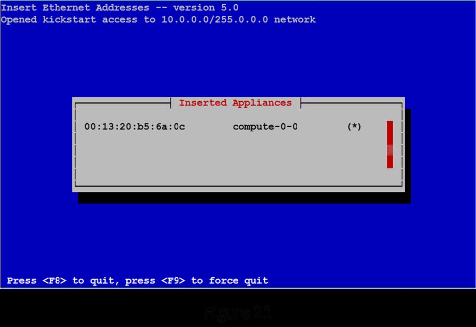
Figure 21. First Node Installing
Install the rest of your compute nodes. After a couple more nodes are booted, the list of installed nodes looks like Figure 22.
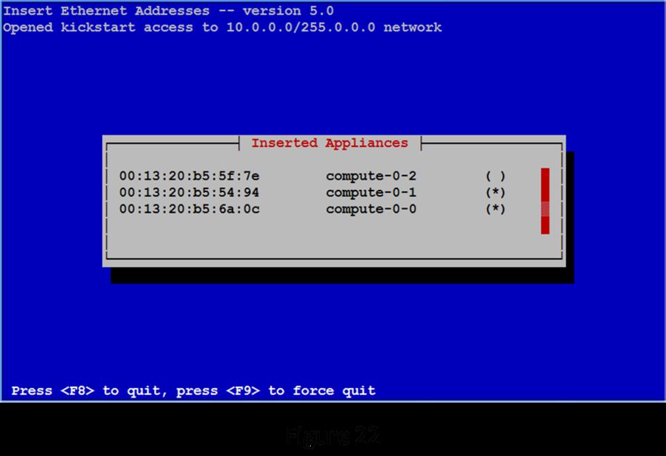
Figure 22. List of Installed Appliances (Three Nodes Added)
When the last node in the cluster reboots at the end of its loading process, press F8 on the head node to finish the installation.
Your cluster now is complete and ready for work. First job: roll call. The Rocks cluster-fork function allows the user to execute the same application on all or a subset of the nodes in the cluster. Figure 23 shows executing the uname command via cluster-fork.
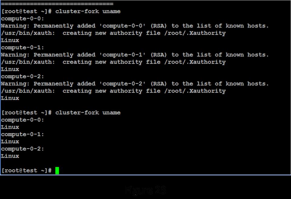
Figure 23. Running uname via cluster-fork
The first invocation requires the system to set up the security for each node. Once this is done, subsequent invocations simply run the application. It appears that all of the nodes in the cluster are healthy and ready for work.
If you are looking for a more comprehensive test, take a look at the Intel Cluster Checker package. This application is useful both on a newly created cluster and as a tool for ongoing maintenance.
Now that your cluster is functional, it's time to show it off. One of the more interesting parallel applications is NAMD, a molecular dynamics simulator from the University of Illinois. Paired with VMD, its graphical interface, you essentially have a chemistry set in your cluster.
When a workstation isn't fast enough, a properly configured cluster can provide all the computing capability you require. Although it is possible to set up a compute cluster manually, many packages are available, both free and commercially supported, that can make the installation and configuration process essentially painless.
