Scale Out with GlusterFS

GlusterFS is an open-source distributed filesystem, originally developed by a small California startup, Gluster Inc. Two years ago, Red Hat acquired Gluster, and today, it sponsors GlusterFS as an open-source product with commercial support, called Red Hat Storage Server. This article refers to the latest community version of GlusterFS for CentOS, which is 3.4 at the time of this writing. The material covered here also applies to Red Hat Storage Server as well as other Linux distributions.

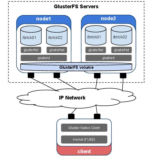
Figure 1. Simplified Architecture Diagram of a Two-Node GlusterFS Cluster and Native Client

Figure 1 shows a simplified architecture of GlusterFS. GlusterFS provides a unified, global namespace that combines the storage resources from multiple servers. Each node in the GlusterFS storage pool exports one or more bricks via the glusterfsd dæmon. Bricks are just local filesystems, usually indicated by the hostname:/directory notation. They are the basic building blocks of a GlusterFS volume, which can be mounted using the GlusterFS Native Client. This typically provides the best performance and is based on the Filesystem In Userspace (FUSE) interface built in to the Linux kernel. GlusterFS also provides object access via the OpenStack Swift API and connectivity through the NFS and CIFS protocols.

You can increase capacity or IOPS in a GlusterFS storage pool by adding more nodes and expanding the existing volumes to include the new bricks. As you provision additional storage nodes, you increase not only the total storage capacity, but network bandwidth, memory and CPU resources as well. GlusterFS scales “out” instead of “up”.

Unlike traditional storage arrays, there is no hard limit provided by the array controller; you are limited by the sum of all your storage nodes. This scalability results in a small latency penalty per I/O operation. Therefore, GlusterFS works very well where nearline storage access is required, such as bandwidth-intensive HPC or general-purpose archival storage. It is less suited for latency-sensitive applications, such as highly transactional databases.

Installing GlusterFS is straightforward. You can download packages for the most common distributions, including CentOS, Fedora, Debian and Ubuntu. For CentOS and other distributions with the yum package manager, just add the corresponding yum repo, as explained in the official GlusterFS Quick Start Guide (see Resources). Then, install the glusterfs-server-* package on the storage servers and glusterfs-client-* on the clients. Finally, start the glusterd service on the storage nodes:

# service glusterd start

The next task is to create a trusted storage pool, which is made from the bricks of the storage nodes. From one of the servers, for instance node1, just type:

# gluster peer probe node2

And, repeat that for all the other storage nodes. The command gluster peer status lists all the other peers and their connection status.

The first step to provision a volume consists of setting up the bricks. As mentioned previously, these are mountpoints on the storage nodes, with XFS being the recommended filesystem. GlusterFS uses extended file attributes to store key/value pairs for several purposes, such as volume replication or striping across different bricks. To make this work with XFS, you should format the bricks using a larger inode size—for example, 512 bytes:

# mkfs.xfs -i 512 /brick01

GlusterFS volumes can belong to several different types. They can be distributed, replicated or striped. In addition, they can be a combination of these—for instance, distributed replicated or striped replicated. You can specify the type of a volume using the stripe and replica keywords of the gluster command. There is no keyword to indicate that a volume is distributed, as this is the default configuration.

Distributed volumes store whole files across different bricks. This is similar to striping, but the minimum “unit of storage” in a brick for a distributed volume is a single file. Conversely, striped volumes split files in chunks (of 128KB by default) and stripe those across bricks. Although striped volumes increase complexity, you might use them if you have very large files that do not fit in a single brick or in scenarios where a lot of file contention is experienced. The last volume type, replicated, provides redundancy by synchronously replicating files across different bricks.

As an example, let's create a distributed replicated volume using the bricks mounted on the /brick01 and /brick02 directories on two different storage nodes:

# gluster volume create MYVOL replica 2 \
> node{1,2}:/brick01 node{1,2}:/brick02
# gluster volume start MYVOL

The replica 2 option tells GlusterFS to dedicate half the bricks for two-way replication. Keep in mind that the order of the bricks does matter. In the previous example, node1:/brick01 will mirror node2:/brick01. The same logic applies to /brick02.

Finally, you can make the new volume available on other machines using the GlusterFS native client:

# mount -t glusterfs node1:/MYVOL /mnt/DIR

You can pass the -o backupvolfile-server option on the previous command to specify an alternative server from which to mount the filesystem, should node1 be unavailable.

GlusterFS offers more flexibility and scalability than a traditional monolithic storage solution. But, this comes at a complexity cost, as you now have more control and need to consider several aspects for best performance.

To check whether performance meets your expectations, start with a baseline benchmark to measure throughput on the newly created GlusterFS volume. You can use several tools to do this, such as iozone, mpirun or dd. For example, run the following script after changing directory into a GlusterFS mountpoint:

#!/bin/bash
for BS in 64 128 256 512 1024 2048 4096 8192 ; do
  iozone -R -b results-${BS}.xls -t 16 -r $BS -s 8g \
    -i 0 -i 1 -i 2
done

The previous code runs iozone with different block sizes and 16 active client threads, using an 8GB file size to test. To minimize the effects of caching, you should benchmark I/O performance using a file size at least twice the RAM installed on your servers. However, as RAM is cheap and many new servers come equipped with a lot of memory, it may be impractical to test with very large file sizes. Instead, you can limit the amount of RAM seen by the kernel to 2GB—for example, by passing the mem=2G kernel option at boot.

Generally, you will discover that throughput is either limited by the network or the storage layer. To identify where the system is constrained, run sar and iostat in separate terminals for each GlusterFS node, as illustrated below:

# sar -n DEV 2 | egrep "(IFACE|eth0|eth1|bond0)"
# iostat -N -t -x 2 | egrep "(Device|brick)"

Keep an eye on the throughput of each network interface reported by the sar command above. Also, monitor the utilization column of the iostat output to check whether any of the bricks are saturated. The commands gluster volume top and gluster volume profile provide many other useful performance metrics. Refer to the documentation on the Gluster community Web site for more details.

Once you have identified where the bottleneck is on your system, you can do some simple tuning.

GlusterFS supports TCP/IP and RDMA as the transport protocols. TCP on IPoIB (IP over InfiniBand) is also a viable option. Due to space limitations, here we mostly refer to TCP/IP over Ethernet, although some considerations also apply to IPoIB.

There are several ways to improve network throughput on your storage servers. You certainly should minimize per-packet overhead and balance traffic across your network interfaces in the most effective way, so that none of the NIC ports are underutilized. Under normal conditions, no particular TCP tuning is required, as the Linux kernel enables TCP window scaling by default and does a good job of automatically adjusting buffer sizes for TCP performance.

To reduce packet overhead, you should put your storage nodes on the same network segment as the clients and enable jumbo frames. To do so, all the interfaces on your network switches and GlusterFS servers must be set up with a larger MTU size. Typically a maximum value of 9,000 bytes is allowed on most switch platforms and network cards.

You also should ensure that TSO (TCP segment offload) or GSO (generic segment offload) is enabled, if supported by the NIC driver. Use the ethtool command with the -k option to verify the current settings. TSO and GSO allow the kernel to manipulate much larger packet sizes and offload to the NIC hardware the process of segmenting packets into smaller frames, thus reducing CPU and packet overhead. Similarly, large receive offload (LRO) and generic receive offload (GRO) can improve throughput in the inbound direction.

Another important aspect to take into consideration is NIC bonding. The Linux bonding driver provides several load-balancing policies, such as active-backup or round-robin. In a GlusterFS setup, an active-backup policy may result in a bottleneck, as only one of the Ethernet interfaces will be used to transmit and receive packets. Conversely, a pure round-robin policy provides per-packet load balancing and full utilization of the bandwidth of all the interfaces if required. However, depending on your network topology, round-robin may cause out-of-order packet delivery, and your system would require extra CPU cycles to re-assemble them.

Better alternatives in this case are IEEE 802.3ad dynamic link aggregation (selected with mode=4 in the bonding driver) or adaptive load balancing (mode=6). To deploy IEEE 802.3ad link aggregation, an essential requirement is that the switches connected to the servers must also support this protocol. Then, the xmit_hash_policy parameter of the Linux kernel bonding driver specifies the hash policy used to balance traffic across the interfaces, when 802.3ad is in operation. For better results, this parameter should be set to layer3+4. This policy uses a hash of the source and destination IP addresses and TCP ports to select the outbound interface. In this way, traffic is load-balanced per flow, rather than per packet, and the end result is that packets from a certain connection socket always will be delivered out of the same network interface.

In GlusterFS, when a client mounts a volume using the native protocol, a TCP connection is established from the client for each brick hosted on the storage nodes. On an eight-node cluster with two bricks per node, this results in 16 TCP connections. Hence, the “layer3+4” hash transmit policy typically would contain enough “entropy” to split those connections evenly across the network interfaces, resulting in an efficient and balanced usage of all the NIC ports.

A final consideration concerns management traffic. For security purposes, you may want to separate GlusterFS and management traffic (such as SSH, SNMP and so on) onto different subnets. To achieve best performance, you also should use different physical interfaces; otherwise, you may get contention between storage and management traffic over the same NIC ports. If your servers come with only two network interfaces, you still can split storage and management traffic onto different subnets by using VLAN tagging.

Figure 2 illustrates a potential configuration to achieve this result. On a server with two physical network ports, we have aggregated those into a bond interface named bond0, for GlusterFS traffic. The corresponding configuration is shown below:

# cat /etc/sysconfig/network-scripts/ifcfg-bond0
DEVICE=bond0
BONDING_OPTS="miimon=100 mode=4 xmit_hash_policy=layer3+4"
MTU=9000
BOOTPROTO=none
IPADDR=192.168.1.1
NETMASK=255.255.255.0

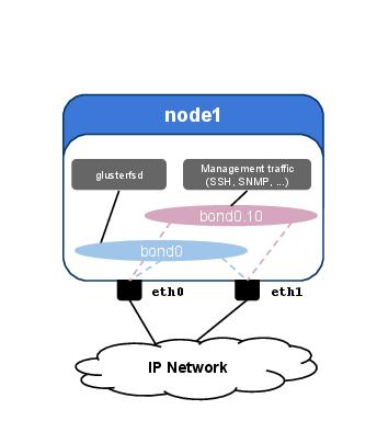
Figure 2. Network Configuration on a GlusterFS Server with Multiple Bond Interfaces and VLAN Tagging

We have also created a second, logical interface named bond0.10. The configuration is listed below:

# cat /etc/sysconfig/network-scripts/ifcfg-bond0.10
DEVICE=bond0.10
ONPARENT=yes
VLAN=10
MTU=1500
IPADDR=10.1.1.1
NETMASK=255.255.255.0
GATEWAY=10.1.1.254

This interface is used for traffic management and is set up with a standard MTU of 1,500 bytes and a VLAN tag. Conversely, bond0 is not set with any VLAN tag, so it will send traffic untagged, which on the switches will be assigned to the native VLAN of the corresponding Ethernet trunk.

As of today, the commodity x86 servers with the highest density of local storage can fit up to 26 local drives in their chassis. If two drives are dedicated to the OS, this leaves 24 drives to host the GlusterFS bricks. You can add additional drives via Direct Attached Storage (DAS), but before scaling “up”, you should check whether you have enough spare network bandwidth. With large sequential I/O patterns, you may run out of bandwidth well before exhausting the throughput of your local drives.

The optimal RAID level and LUN size depend on your workload. If your application generates lots of random write I/O, you may consider aggregating all the drives in a single RAID 10 volume. However, efficiency won't be the best, as you will lose 50% of your capacity. On the other hand, you can go with a RAID 0 configuration for maximum efficiency and performance, and rely on GlusterFS to provide data redundancy via its replication capabilities.

It is not surprising that the best approach often lies in the middle. With 24 drives per node, Red Hat's recommended setup consists of 2 x RAID 6 (10+2) volumes (see Resources). A single volume with a RAID 50 or 60 configuration also can provide similar performance.

On a LUN spanning a RAID 6 volume of 12 SAS hard disk drives, a typical sustained throughput is 1–2GB per second, depending on the type and model of the disk drives. To transfer this amount of data across the network, a single 10Gbps interface easily would become a bottleneck. That's why you should load-balance traffic across your network interfaces, as we discussed previously.

It is important to configure a local LUN volume properly to get the most of the parallel access benefits provided by the RAID controller. The chunk size (often referred to as element stripe size) is the “atomic” block of data that the RAID controller can write to each disk drive before moving onto the next one. If the average I/O request size issued by an application is smaller than the chunk size, only one drive at a time would handle most of the I/O.

The optimal chunk size is obtained by dividing the average I/O request size by the number of data-bearing disks. As an example, a RAID 6 (10+2) volume configuration gives ten data-bearing disks. If the average I/O request issued by your application is 1MB, this gives a chunk size (approximated to the nearest power of 2) of 128KB. Then, the minimum amount of data that the RAID controller distributes across the drives is given by the number of data-bearing disks multiplied by the chunk size. That is, in this example, 10 x 128 KB = 1280 KB, slightly larger than the average I/O request of 1MB that we initially assumed.

Next, ensure that LVM properly aligns its metadata based on the stripe value that was just calculated:

# pvcreate --dataalignment=1280k /dev/sdb

When formatting the bricks, mkfs can optimize the distribution of the filesystem metadata by taking into account the layout of the underlying RAID volume. To do this, pass the su and sw parameters to mkfs.xfs. These indicate the chunk size in bytes and the stripe width as a multiplier of the chunk size, respectively:

# mkfs.xfs -d su=128k,sw=10 -i 512 /brick01

Another setting to consider is the default read ahead of the brick devices. This tells the kernel and RAID controller how much data to pre-fetch when sequential requests come in. The actual value for the kernel is available in the /sys virtual filesystem and is set to 128KB by default:

# cat /sys/block/sdb/queue/read_ahead_kb
128

A typical SAS hard drive with 15k RPM of rotational speed has a standard average response time of around 5ms and can read 128KB (the default read ahead) in less than a millisecond. Under I/O contention, the drive may spend most of its time positioning to a new sector for the next I/O request and use only a small fraction of its time to transfer data. In such situations, a larger read ahead can improve performance. The rationale behind this change is that it is better to pre-fetch a big chunk of data in the hope that it will be used later, as this will reduce the overall seek time of the drives.

Again, there is no optimal value for all workloads, but as a starting point, it may be worth noting that Red Hat recommends to set this parameter to 64MB. However, if your application I/O profile is IOPS-intensive and mostly made of small random requests, you may be better off tuning the read ahead size to a lower value and deploying solid disk drives. The commercial version of GlusterFS provides a built-in profile for the tuned dæmon, which automatically increases read ahead to 64MB and configures the bricks to use the deadline I/O elevator.

GlusterFS is a versatile distributed filesystem, well supported on standard Linux distributions. It is trivial to install and simple to tune, as we have shown here. However, this article is merely a short introduction. We did not have space to cover many of the most exciting features of GlusterFS, such as asynchronous replication, OpenStack Swift integration and CIFS/NFS exports—to mention just a few! We hope this article enables you to give GlusterFS a go in your own environment and explore some of its many capabilities in more detail.